GroupPlots

Create multiple subplots in a grid layout using GroupPlot and NextGroupPlot.

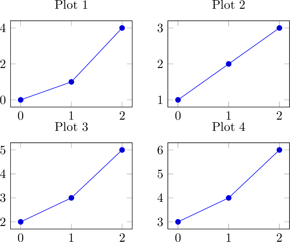
Basic 2x2 Grid

from texer import PGFPlot, GroupPlot, NextGroupPlot, AddPlot, Coordinates, evaluate

plot = PGFPlot(
    GroupPlot(
        group_size="2 by 2",
        plots=[
            NextGroupPlot(
                title="Plot 1",
                plots=[AddPlot(coords=Coordinates([(0, 0), (1, 1), (2, 4)]))],
            ),
            NextGroupPlot(
                title="Plot 2",
                plots=[AddPlot(coords=Coordinates([(0, 1), (1, 2), (2, 3)]))],
            ),
            NextGroupPlot(
                title="Plot 3",
                plots=[AddPlot(coords=Coordinates([(0, 2), (1, 3), (2, 5)]))],
            ),
            NextGroupPlot(
                title="Plot 4",
                plots=[AddPlot(coords=Coordinates([(0, 3), (1, 4), (2, 6)]))],
            ),
        ],
    )
)

print(evaluate(plot, {}))

Understanding the Structure

PGFPlot
└── GroupPlot (grid container)
    ├── group_size: "2 by 2"
    ├── Common options (applied to all subplots)
    └── plots: [NextGroupPlot, NextGroupPlot, ...]
        └── NextGroupPlot (individual subplot)
            ├── Per-subplot options
            └── plots: [AddPlot, ...]

Group Size

Specify grid dimensions with group_size:

group_size="2 by 2"   # 2 columns, 2 rows
group_size="3 by 1"   # 3 columns, 1 row
group_size="1 by 4"   # 1 column, 4 rows

Subplots are filled left-to-right, top-to-bottom.

Common Options

Apply options to all subplots at the GroupPlot level:

GroupPlot(
    group_size="2 by 1",

    # Common axis options (applied to all subplots)
    width="6cm",
    height="4cm",
    grid=True,
    xmin=0,
    xmax=10,

    plots=[...],
)

Individual Subplot Options

Each NextGroupPlot can have its own options:

GroupPlot(
    group_size="1 by 2",
    plots=[
        NextGroupPlot(
            title="Linear Scale",
            xlabel="X",
            ylabel="Y",
            grid=True,
            plots=[AddPlot(coords=Coordinates([(0, 1), (1, 10), (2, 100)]))],
        ),
        NextGroupPlot(
            title="Log Scale",
            xlabel="X",
            ylabel="log(Y)",
            ymin=0.1,
            ymax=1000,
            plots=[AddPlot(coords=Coordinates([(0, 1), (1, 10), (2, 100)]))],
        ),
    ],
)

Spacing and Layout

Control spacing between subplots:

GroupPlot(
    group_size="2 by 2",
    horizontal_sep="2cm",   # Space between columns
    vertical_sep="1.5cm",   # Space between rows
    plots=[...],
)

Label Positioning

Position labels at grid edges for cleaner layouts:

GroupPlot(
    group_size="2 by 2",
    xlabels_at="edge bottom",  # X labels only on bottom row
    ylabels_at="edge left",    # Y labels only on left column
    plots=[
        NextGroupPlot(xlabel="Time", ylabel="Value", plots=[...]),
        NextGroupPlot(xlabel="Time", ylabel="Value", plots=[...]),
        NextGroupPlot(xlabel="Time", ylabel="Value", plots=[...]),
        NextGroupPlot(xlabel="Time", ylabel="Value", plots=[...]),
    ],
)

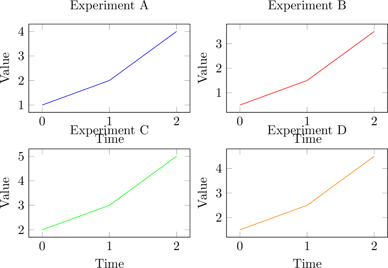
Dynamic GroupPlots with Ref

Generate subplots from data:

from texer import PGFPlot, GroupPlot, NextGroupPlot, AddPlot, Coordinates, Ref, Iter, evaluate

plot = PGFPlot(
    GroupPlot(
        group_size=Ref("grid_size"),
        width="6cm",
        height="4cm",
        plots=Iter(
            Ref("subplots"),
            template=NextGroupPlot(
                title=Ref("title"),
                xlabel=Ref("xlabel"),
                ylabel=Ref("ylabel"),
                plots=[
                    AddPlot(
                        color=Ref("color"),
                        coords=Coordinates(
                            Iter(Ref("data"), x=Ref("x"), y=Ref("y"))
                        ),
                    )
                ],
            )
        ),
    )
)

data = {
    "grid_size": "2 by 2",
    "subplots": [
        {
            "title": "Experiment A",
            "xlabel": "Time",
            "ylabel": "Value",
            "color": "blue",
            "data": [{"x": 0, "y": 1}, {"x": 1, "y": 2}, {"x": 2, "y": 4}],
        },
        {
            "title": "Experiment B",
            "xlabel": "Time",
            "ylabel": "Value",
            "color": "red",
            "data": [{"x": 0, "y": 0.5}, {"x": 1, "y": 1.5}, {"x": 2, "y": 3.5}],
        },
        {
            "title": "Experiment C",
            "xlabel": "Time",
            "ylabel": "Value",
            "color": "green",
            "data": [{"x": 0, "y": 2}, {"x": 1, "y": 3}, {"x": 2, "y": 5}],
        },
        {
            "title": "Experiment D",
            "xlabel": "Time",
            "ylabel": "Value",
            "color": "orange",
            "data": [{"x": 0, "y": 1.5}, {"x": 1, "y": 2.5}, {"x": 2, "y": 4.5}],
        },
    ],
}

print(evaluate(plot, data))

Multiple Series per Subplot

Each subplot can have multiple data series:

GroupPlot(
    group_size="1 by 2",
    plots=[
        NextGroupPlot(
            title="Sensors A & B",
            plots=[
                AddPlot(color="blue", mark="*", coords=Coordinates([...])),
                AddPlot(color="red", mark="square*", coords=Coordinates([...])),
            ],
            legend=["Sensor A", "Sensor B"],
        ),
        NextGroupPlot(
            title="Sensors C & D",
            plots=[
                AddPlot(color="green", mark="*", coords=Coordinates([...])),
                AddPlot(color="orange", mark="square*", coords=Coordinates([...])),
            ],
            legend=["Sensor C", "Sensor D"],
        ),
    ],
)

Shared Axis Ranges

Set common axis ranges for all subplots:

GroupPlot(
    group_size="2 by 2",
    # Shared ranges
    xmin=0,
    xmax=10,
    ymin=0,
    ymax=100,
    plots=[
        NextGroupPlot(title="Plot 1", plots=[...]),
        NextGroupPlot(title="Plot 2", plots=[...]),
        NextGroupPlot(title="Plot 3", plots=[...]),
        NextGroupPlot(title="Plot 4", plots=[...]),
    ],
)

Individual subplots can override these:

plots=[
    NextGroupPlot(title="Plot 1", plots=[...]),  # Uses shared ranges
    NextGroupPlot(
        title="Plot 2",
        ymin=-50,  # Override shared ymin
        ymax=150,  # Override shared ymax
        plots=[...],
    ),
]

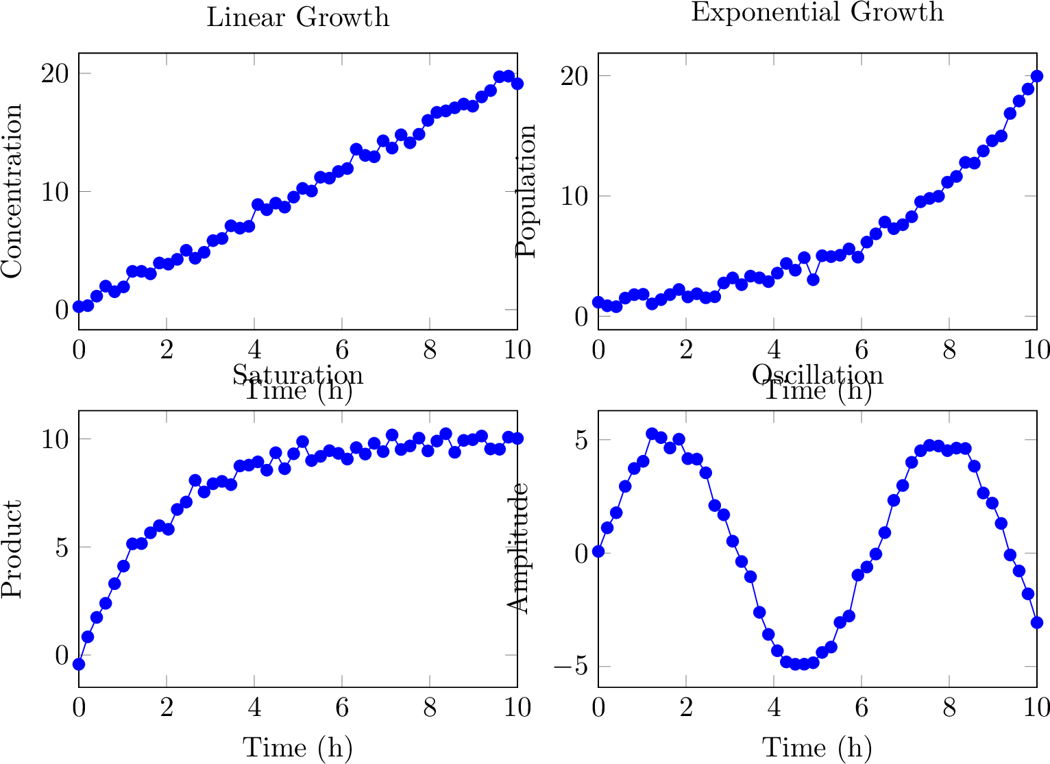
Real-World Example: Comparing Experiments

import numpy as np
from texer import PGFPlot, GroupPlot, NextGroupPlot, AddPlot, Coordinates, Ref, Iter, evaluate

plot = PGFPlot(
    GroupPlot(
        group_size="2 by 2",
        width="7cm",
        height="5cm",
        xmin=0,
        xmax=10,
        grid=True,
        xlabels_at="edge bottom",
        ylabels_at="edge left",
        plots=Iter(
            Ref("experiments"),
            template=NextGroupPlot(
                title=Ref("name"),
                xlabel=Ref("xlabel"),
                ylabel=Ref("ylabel"),
                plots=[
                    AddPlot(
                        color="blue",
                        mark="*",
                        coords=Coordinates(x=Ref("x"), y=Ref("y")),
                    )
                ],
            )
        ),
    )
)

# Generate data for 4 experiments
x = np.linspace(0, 10, 50)
data = {
    "experiments": [
        {
            "name": "Linear Growth",
            "xlabel": "Time (h)",
            "ylabel": "Concentration",
            "x": x,
            "y": 2 * x + np.random.normal(0, 0.5, len(x)),
        },
        {
            "name": "Exponential Growth",
            "xlabel": "Time (h)",
            "ylabel": "Population",
            "x": x,
            "y": np.exp(0.3 * x) + np.random.normal(0, 0.5, len(x)),
        },
        {
            "name": "Saturation",
            "xlabel": "Time (h)",
            "ylabel": "Product",
            "x": x,
            "y": 10 * (1 - np.exp(-0.5 * x)) + np.random.normal(0, 0.3, len(x)),
        },
        {
            "name": "Oscillation",
            "xlabel": "Time (h)",
            "ylabel": "Amplitude",
            "x": x,
            "y": 5 * np.sin(x) + np.random.normal(0, 0.3, len(x)),
        },
    ]
}

print(evaluate(plot, data))

Legends in GroupPlots

Each subplot can have its own legend:

NextGroupPlot(
    title="Sensor Comparison",
    plots=[
        AddPlot(color="blue", coords=Coordinates([...])),
        AddPlot(color="red", coords=Coordinates([...])),
    ],
    legend=["Sensor A", "Sensor B"],
    legend_pos="north east",
)

Mixing Plot Types

Different subplots can have different plot types:

GroupPlot(
    group_size="2 by 1",
    plots=[
        NextGroupPlot(
            title="Scatter Plot",
            plots=[
                AddPlot(
                    color="blue",
                    mark="o",
                    only_marks=True,
                    coords=Coordinates([...]),
                )
            ],
        ),
        NextGroupPlot(
            title="Line Plot",
            plots=[
                AddPlot(
                    color="red",
                    thick=True,
                    no_marks=True,
                    coords=Coordinates([...]),
                )
            ],
        ),
    ],
)

Empty Subplots

If you have fewer plots than grid cells, the remaining cells are left empty:

GroupPlot(
    group_size="2 by 2",
    plots=[
        NextGroupPlot(title="Plot 1", plots=[...]),
        NextGroupPlot(title="Plot 2", plots=[...]),
        NextGroupPlot(title="Plot 3", plots=[...]),
        # Fourth cell is empty
    ],
)

With Cycle Lists

Apply a cycle list to all subplots:

GroupPlot(
    group_size="2 by 2",
    cycle_list=[
        {"color": "blue", "mark": "*"},
        {"color": "red", "mark": "square*"},
    ],
    plots=[
        NextGroupPlot(
            title="Subplot 1",
            plots=[
                AddPlot(coords=Coordinates([...])),  # Gets blue, *
                AddPlot(coords=Coordinates([...])),  # Gets red, square*
            ],
        ),
        NextGroupPlot(
            title="Subplot 2",
            plots=[
                AddPlot(coords=Coordinates([...])),  # Gets blue, *
                AddPlot(coords=Coordinates([...])),  # Gets red, square*
            ],
        ),
    ],
)

See Advanced Options - Cycle Lists for more details.

Comparison with Shared Legend

Create a shared legend for all subplots using raw LaTeX:

from texer import Raw

GroupPlot(
    group_size="2 by 2",
    plots=[
        NextGroupPlot(plots=[
            AddPlot(color="blue", coords=Coordinates([...])),
            AddPlot(color="red", coords=Coordinates([...])),
        ]),
        NextGroupPlot(plots=[
            AddPlot(color="blue", coords=Coordinates([...])),
            AddPlot(color="red", coords=Coordinates([...])),
        ]),
        NextGroupPlot(plots=[
            AddPlot(color="blue", coords=Coordinates([...])),
            AddPlot(color="red", coords=Coordinates([...])),
        ]),
        NextGroupPlot(
            plots=[
                AddPlot(color="blue", coords=Coordinates([...])),
                AddPlot(color="red", coords=Coordinates([...])),
            ],
            legend=["Series A", "Series B"],
            legend_pos="south east",
        ),
    ],
)

The legend from the last subplot serves as a shared legend since all use the same colors.

Performance Tips

For large grids with many data points:

1. Reduce samples: Use fewer points per plot
2. Disable markers: Use no_marks=True for line plots
3. Share data: Use references to avoid duplicating large arrays
4. Limit grid size: Keep grids under 4x4 for best performance

Next Steps

• Multiple Series - Multiple series within plots
• Advanced Options - Cycle lists and advanced styling
• Data-Driven Plots - Dynamic plot generation