3D Surface Plots
PGFPlots supports 3D surface and mesh plots for visualizing functions of two variables.
Mental Model for 3D Plots
3D plots build on the same structure as 2D plots, with additional dimensions:
PGFPlot (tikzpicture wrapper)
└── Axis (3D coordinate system)
    ├── Options (xlabel, ylabel, zlabel, view, colorbar, ...)
    └── AddPlot with surf or mesh
        ├── 3D coordinates (x, y, z)
        └── Style options
- Axis: Same as 2D, but with
zlabel,zmin,zmaxfor the third dimension - AddPlot: Use
surf=Truefor surface plots ormesh=Truefor mesh plots - Coordinates: Provide
x,y, andzdata - View: Control the viewing angle with the
viewoption
Your First 3D Surface Plot
Let's create a simple 3D surface plot using NumPy to generate data:
import numpy as np
from texer import PGFPlot, Axis, AddPlot, Coordinates, evaluate

# Generate mesh grid
x = np.linspace(-3, 3, 30)
y = np.linspace(-3, 3, 30)
X, Y = np.meshgrid(x, y)

# Calculate Z values (a simple paraboloid)
Z = X**2 + Y**2

# Flatten for coordinates
x_flat = X.flatten()
y_flat = Y.flatten()
z_flat = Z.flatten()

plot = PGFPlot(
    Axis(
        xlabel="X",
        ylabel="Y",
        zlabel="Z",
        plots=[
            AddPlot(
                surf=True,  # Use surf for filled surface
                coords=Coordinates(x=x_flat, y=y_flat, z=z_flat),
            )
        ],
        _raw_options="colorbar",  # Add a colorbar
    )
)

print(evaluate(plot, {}))
LaTeX code
Surface vs Mesh
Surface Plot (surf=True)
Surface plots show filled surfaces with colors representing height:
import numpy as np
from texer import PGFPlot, Axis, AddPlot, Coordinates, evaluate

# Generate data
x = np.linspace(-2, 2, 20)
y = np.linspace(-2, 2, 20)
X, Y = np.meshgrid(x, y)
Z = np.sin(np.sqrt(X**2 + Y**2))

plot = PGFPlot(
    Axis(
        xlabel="X",
        ylabel="Y",
        zlabel="Z",
        plots=[
            AddPlot(
                surf=True,
                coords=Coordinates(
                    x=X.flatten(),
                    y=Y.flatten(),
                    z=Z.flatten()
                ),
            )
        ],
    )
)
Mesh Plot (mesh=True)
Mesh plots show wireframe surfaces:
plot = PGFPlot(
    Axis(
        xlabel="X",
        ylabel="Y",
        zlabel="Z",
        plots=[
            AddPlot(
                mesh=True,  # Wireframe instead of filled
                coords=Coordinates(
                    x=X.flatten(),
                    y=Y.flatten(),
                    z=Z.flatten()
                ),
            )
        ],
    )
)
Common 3D Surface Examples
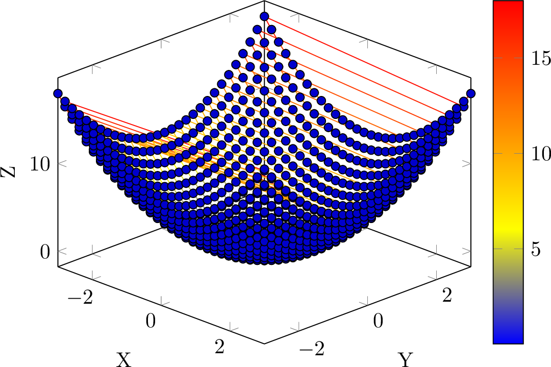
Paraboloid
import numpy as np
from texer import PGFPlot, Axis, AddPlot, Coordinates, evaluate

x = np.linspace(-3, 3, 25)
y = np.linspace(-3, 3, 25)
X, Y = np.meshgrid(x, y)
Z = X**2 + Y**2

plot = PGFPlot(
    Axis(
        xlabel="X",
        ylabel="Y",
        zlabel="$Z = X^2 + Y^2$",
        plots=[
            AddPlot(
                surf=True,
                coords=Coordinates(x=X.flatten(), y=Y.flatten(), z=Z.flatten()),
            )
        ],
        _raw_options="colorbar",
    )
)
Sinc Function
import numpy as np
from texer import PGFPlot, Axis, AddPlot, Coordinates, evaluate

x = np.linspace(-5, 5, 30)
y = np.linspace(-5, 5, 30)
X, Y = np.meshgrid(x, y)
R = np.sqrt(X**2 + Y**2) + 1e-10  # Avoid division by zero
Z = np.sin(R) / R  # Sinc function

plot = PGFPlot(
    Axis(
        xlabel="X",
        ylabel="Y",
        zlabel="$\\text{sinc}(r)$",
        plots=[
            AddPlot(
                surf=True,
                coords=Coordinates(x=X.flatten(), y=Y.flatten(), z=Z.flatten()),
            )
        ],
        _raw_options="colorbar, view={45}{30}",  # Set viewing angle
    )
)
Saddle Surface
import numpy as np
from texer import PGFPlot, Axis, AddPlot, Coordinates, evaluate

x = np.linspace(-2, 2, 25)
y = np.linspace(-2, 2, 25)
X, Y = np.meshgrid(x, y)
Z = X**2 - Y**2  # Saddle surface (hyperbolic paraboloid)

plot = PGFPlot(
    Axis(
        xlabel="X",
        ylabel="Y",
        zlabel="$Z = X^2 - Y^2$",
        plots=[
            AddPlot(
                surf=True,
                coords=Coordinates(x=X.flatten(), y=Y.flatten(), z=Z.flatten()),
            )
        ],
        _raw_options="colorbar",
    )
)
Customization Options
Viewing Angle
Control the 3D viewing angle with the view option:
plot = PGFPlot(
    Axis(
        xlabel="X",
        ylabel="Y",
        zlabel="Z",
        plots=[AddPlot(surf=True, coords=...)],
        _raw_options="view={60}{30}",  # azimuth=60°, elevation=30°
    )
)
Common viewing angles:
- view={45}{30} - Default perspective (45° azimuth, 30° elevation)
- view={0}{90} - Top-down view (looking along Z axis)
- view={0}{0} - Side view (looking along Y axis)
- view={90}{0} - Front view (looking along X axis)
Colorbar
Add a colorbar to show the color scale:
plot = PGFPlot(
    Axis(
        plots=[AddPlot(surf=True, coords=...)],
        _raw_options="colorbar",  # Add colorbar
    )
)
You can also customize the colorbar:
plot = PGFPlot(
    Axis(
        plots=[AddPlot(surf=True, coords=...)],
        _raw_options="colorbar, colorbar horizontal",  # Horizontal colorbar
    )
)
Color Maps
PGFPlots supports various color maps:
plot = PGFPlot(
    Axis(
        plots=[AddPlot(surf=True, coords=...)],
        _raw_options="colormap/hot, colorbar",  # Use 'hot' colormap
    )
)
Common colormaps:
- hot - Black → red → yellow → white
- cool - Cyan → magenta
- bluered - Blue → red
- greenyellow - Green → yellow
- redyellow - Red → yellow
- viridis - Perceptually uniform colormap
- jet - Blue → cyan → yellow → red (classic MATLAB)
Axis Limits
Control the visible range:
plot = PGFPlot(
    Axis(
        xlabel="X",
        ylabel="Y",
        zlabel="Z",
        xmin=-3, xmax=3,
        ymin=-3, ymax=3,
        zmin=0, zmax=10,
        plots=[AddPlot(surf=True, coords=...)],
    )
)
Data-Driven 3D Plots
Use Ref and Iter for dynamic 3D surfaces:
from texer import PGFPlot, Axis, AddPlot, Coordinates, Ref, evaluate
import numpy as np

plot = PGFPlot(
    Axis(
        xlabel=Ref("x_label"),
        ylabel=Ref("y_label"),
        zlabel=Ref("z_label"),
        plots=[
            AddPlot(
                surf=True,
                coords=Coordinates(
                    x=Ref("x_data"),
                    y=Ref("y_data"),
                    z=Ref("z_data"),
                ),
            )
        ],
        _raw_options=Ref("plot_options"),
    )
)

# Generate data
x = np.linspace(-2, 2, 20)
y = np.linspace(-2, 2, 20)
X, Y = np.meshgrid(x, y)
Z = X * np.exp(-X**2 - Y**2)

data = {
    "x_label": "X",
    "y_label": "Y",
    "z_label": "Z",
    "x_data": X.flatten(),
    "y_data": Y.flatten(),
    "z_data": Z.flatten(),
    "plot_options": "colorbar, view={45}{30}",
}

print(evaluate(plot, data))
Tips for 3D Plots
Data Format
For surface plots, provide data as flattened 1D arrays. PGFPlots will automatically reconstruct the surface from the coordinate order.
Resolution
More points create smoother surfaces but increase compilation time. Start with 20-30 points per dimension, then increase if needed.
Coordinate Precision
The Coordinates class uses precision=6 by default to round values. For large datasets, this keeps LaTeX files manageable. Adjust with precision=N or precision=None for no rounding.
Compilation Time
3D surface plots can be slow to compile with pdflatex. Consider:
- Reducing the number of points
- Using lualatex instead of pdflatex for better performance
- Caching compiled plots when possible
Mathematical Functions
For plotting mathematical expressions directly, use PGFPlots' expression syntax:
However, NumPy-based approaches give you more control over data preprocessing.Next Steps
- Basic Plots - 2D plotting fundamentals
- Advanced Options - Cycle lists, legends, and customization
- GroupPlots - Multiple subplots in a grid
- Data-Driven Plots - Use specs for dynamic plots