Card-Heining-Kline event study example

# Add PyTwoWay to system path (do not run this)
# import sys
# sys.path.append('../../..')

Import the PyTwoWay package

Make sure to install it using pip install pytwoway.

import pytwoway as tw
import bipartitepandas as bpd

Get your data ready

For this notebook, we simulate data.

df = bpd.SimBipartite().simulate()
display(df)

	i	j	y	t	l	k	alpha	psi
0	0	81	0.283938	0	2	4	0.000000	-0.114185
1	0	81	-1.613504	1	2	4	0.000000	-0.114185
2	0	175	1.057488	2	2	8	0.000000	0.908458
3	0	45	0.894313	3	2	2	0.000000	-0.604585
4	0	90	1.122351	4	2	4	0.000000	-0.114185
...	...	...	...	...	...	...	...	...
49995	9999	2	-2.978308	0	0	0	-0.967422	-1.335178
49996	9999	2	-2.532244	1	0	0	-0.967422	-1.335178
49997	9999	14	-2.428863	2	0	0	-0.967422	-1.335178
49998	9999	14	-0.928106	3	0	0	-0.967422	-1.335178
49999	9999	21	-3.030404	4	0	1	-0.967422	-0.908458

50000 rows × 8 columns

Prepare data

This is exactly how you should prepare real data prior to generating the CHK plot.

• First, we convert the data into a BipartitePandas DataFrame

• Second, we clean the data (e.g. drop NaN observations, make sure firm and worker ids are contiguous, etc.)

• Third, we cluster firms by the quartile of their mean income, to generate firm classes (columns g1 and g2). Alternatively, manually set the columns g1 and g2 to pre-estimated clusters (but make sure to add them correctly!).

• Fourth, we convert the data into extended event study format

Further details on BipartitePandas can be found in the package documentation, available here.

Note

In general, the CHK event study is generated by clustering the data using quartiles of firm-level mean income.

measures = bpd.measures.Moments(measures='mean')
grouping = bpd.grouping.Quantiles(n_quantiles=4)
cluster_params = bpd.cluster_params(
    {
        'measures': measures,
        'grouping': grouping
    }
)

bdf = bpd.BipartiteDataFrame(
    i=df['i'], j=df['j'], y=df['y'], t=df['t']
) \
    .clean() \
    .cluster(cluster_params) \
    .to_extendedeventstudy(transition_col='j', periods_pre=2, periods_post=2)

checking required columns and datatypes
sorting rows
dropping NaN observations
generating 'm' column
keeping highest paying job for i-t (worker-year) duplicates (how='max')
dropping workers who leave a firm then return to it (how=False)
making 'i' ids contiguous
making 'j' ids contiguous
computing largest connected set (how=None)
sorting columns
resetting index

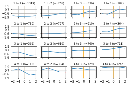
Creating CHK event study plot

Once the data is cleaned, clustered, and in extended event study form, we can generate the event study plots.

tw.diagnostics.plot_extendedeventstudy(bdf, periods_pre=2, periods_post=2)

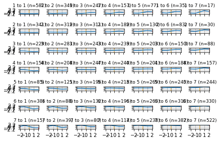
Warning

Be careful not to include too many clusters!

measures = bpd.measures.Moments(measures='mean')
grouping = bpd.grouping.Quantiles(n_quantiles=7)
cluster_params = bpd.cluster_params(
    {
        'measures': measures,
        'grouping': grouping
    }
)

bdf = bpd.BipartiteDataFrame(
    i=df['i'], j=df['j'], y=df['y'], t=df['t']
) \
    .clean() \
    .cluster(cluster_params) \
    .to_extendedeventstudy(transition_col='j', periods_pre=2, periods_post=2)

tw.diagnostics.plot_extendedeventstudy(bdf, periods_pre=2, periods_post=2)

checking required columns and datatypes
sorting rows
dropping NaN observations
generating 'm' column
keeping highest paying job for i-t (worker-year) duplicates (how='max')
dropping workers who leave a firm then return to it (how=False)
making 'i' ids contiguous
making 'j' ids contiguous
computing largest connected set (how=None)
sorting columns
resetting index