BLM example
[1]:
# Add PyTwoWay to system path (do not run this)
# import sys
# sys.path.append('../../..')
Import the PyTwoWay package
Make sure to install it using pip install pytwoway.
[2]:
import numpy as np
import bipartitepandas as bpd
import pytwoway as tw
from pytwoway import constraints as cons
from matplotlib import pyplot as plt
First, check out parameter options
Do this by running:
BLM -
tw.blm_params().describe_all()Clustering -
bpd.cluster_params().describe_all()Cleaning -
bpd.clean_params().describe_all()Simulating -
bpd.sim_params().describe_all()
Alternatively, run x_params().keys() to view all the keys for a parameter dictionary, then x_params().describe(key) to get a description for a single key.
Second, set parameter choices
[3]:
nl = 3 # Number of worker types
nk = 4 # Number of firm types
blm_params = tw.blm_params({
    'nl': nl, 'nk': nk,
    'a1_mu': 0, 'a1_sig': 1.5, 'a2_mu': 0, 'a2_sig': 1.5,
    's1_low': 0.5, 's1_high': 1.5, 's2_low': 0.5, 's2_high': 1.5
})
cluster_params = bpd.cluster_params({
    'measures': bpd.measures.CDFs(),
    'grouping': bpd.grouping.KMeans(n_clusters=nk),
    'is_sorted': True,
    'copy': False
})
clean_params = bpd.clean_params({
    'drop_returns': 'returners',
    'copy': False
})
sim_params = bpd.sim_params({
    'nl': nl, 'nk': nk,
    'alpha_sig': 1, 'psi_sig': 1, 'w_sig': 0.6,
    'c_sort': 0, 'c_netw': 0, 'c_sig': 1
})
Extract data (we simulate for the example)
BipartitePandas contains the class SimBipartite which we use here to simulate a bipartite network. If you have your own data, you can import it during this step. Load it as a Pandas DataFrame and then convert it into a BipartitePandas DataFrame in the next step.
Note that l gives the true worker type and k gives the true firm type, while alpha gives the true worker effect and psi gives the true firm effect. We will save these columns separately.
The BLM estimator uses the firm types computed via clustering, which are saved in columns g1 and g2.
[4]:
sim_data = bpd.SimBipartite(sim_params).simulate()
Prepare data
This is exactly how you should prepare real data prior to running the BLM estimator.
First, we convert the data into a
BipartitePandas DataFrameSecond, we clean the data (e.g. drop NaN observations, make sure firm and worker ids are contiguous, etc.)
Third, we cluster firms by their wage distributions, to generate firm classes (columns
g1andg2). Alternatively, manually set the columnsg1andg2to pre-estimated clusters (but make sure to add them correctly!).Fourth, we collapse the data at the worker-firm spell level (taking mean wage over the spell)
Fifth, we convert the data into event study format
Further details on BipartitePandas can be found in the package documentation, available here.
[5]:
# Convert into BipartitePandas DataFrame
sim_data = bpd.BipartiteDataFrame(sim_data)
# Clean and collapse
sim_data = sim_data.clean(clean_params).collapse(is_sorted=True, copy=False)
# Cluster
sim_data = sim_data.cluster(cluster_params)
# Convert to event study format
sim_data = sim_data.to_eventstudy(is_sorted=True, copy=False)
checking required columns and datatypes
sorting rows
dropping NaN observations
generating 'm' column
keeping highest paying job for i-t (worker-year) duplicates (how='max')
dropping workers who leave a firm then return to it (how='returners')
making 'i' ids contiguous
making 'j' ids contiguous
computing largest connected set (how=None)
sorting columns
resetting index
Separate observed and unobserved data
Some of the simulated data is not observed, so we separate out that data during estimation.
[6]:
sim_data_observed = sim_data.loc[:, ['i', 'j1', 'j2', 'y1', 'y2', 't11', 't12', 't21', 't22', 'g1', 'g2', 'w1', 'w2', 'm']]
sim_data_unobserved = sim_data.loc[:, ['alpha1', 'alpha2', 'k1', 'k2', 'l1', 'l2', 'psi1', 'psi2']]
Separate movers and stayers data
We need to distinguish movers and stayers for the estimator.
[7]:
movers = sim_data_observed.get_worker_m(is_sorted=True)
jdata = sim_data_observed.loc[movers, :]
sdata = sim_data_observed.loc[~movers, :]
Check the data
Let’s check the cleaned data.
[8]:
print('Movers data')
display(jdata)
print('Stayers data')
display(sdata)
Movers data
| i | j1 | j2 | y1 | y2 | t11 | t12 | t21 | t22 | g1 | g2 | w1 | w2 | m | |
|---|---|---|---|---|---|---|---|---|---|---|---|---|---|---|
| 0 | 0 | 189 | 141 | 0.658481 | -0.302737 | 0 | 0 | 1 | 3 | 0 | 3 | 1 | 3 | 1 |
| 1 | 0 | 141 | 179 | -0.302737 | -0.070679 | 1 | 3 | 4 | 4 | 3 | 0 | 3 | 1 | 1 |
| 2 | 1 | 3 | 178 | -0.977635 | -0.138164 | 0 | 0 | 1 | 4 | 1 | 0 | 1 | 4 | 1 |
| 3 | 2 | 179 | 9 | 0.273751 | -2.872666 | 0 | 2 | 3 | 3 | 0 | 1 | 3 | 1 | 1 |
| 4 | 2 | 9 | 113 | -2.872666 | -1.395046 | 3 | 3 | 4 | 4 | 1 | 3 | 1 | 1 | 1 |
| ... | ... | ... | ... | ... | ... | ... | ... | ... | ... | ... | ... | ... | ... | ... |
| 20331 | 9923 | 5 | 18 | -2.439280 | -2.086203 | 0 | 0 | 1 | 1 | 1 | 1 | 1 | 1 | 1 |
| 20332 | 9923 | 18 | 186 | -2.086203 | 0.518828 | 1 | 1 | 2 | 2 | 1 | 0 | 1 | 1 | 1 |
| 20333 | 9923 | 186 | 92 | 0.518828 | 0.440968 | 2 | 2 | 3 | 3 | 0 | 2 | 1 | 1 | 1 |
| 20334 | 9923 | 92 | 14 | 0.440968 | -1.070705 | 3 | 3 | 4 | 4 | 2 | 1 | 1 | 1 | 1 |
| 20335 | 9924 | 167 | 42 | 1.730241 | -0.256907 | 0 | 0 | 1 | 4 | 0 | 1 | 1 | 4 | 1 |
19695 rows × 14 columns
Stayers data
| i | j1 | j2 | y1 | y2 | t11 | t12 | t21 | t22 | g1 | g2 | w1 | w2 | m | |
|---|---|---|---|---|---|---|---|---|---|---|---|---|---|---|
| 16 | 9 | 183 | 183 | 1.775003 | 1.775003 | 0 | 4 | 0 | 4 | 0 | 0 | 5 | 5 | 0 |
| 101 | 55 | 36 | 36 | -0.154698 | -0.154698 | 0 | 4 | 0 | 4 | 1 | 1 | 5 | 5 | 0 |
| 127 | 65 | 192 | 192 | 0.476397 | 0.476397 | 0 | 4 | 0 | 4 | 0 | 0 | 5 | 5 | 0 |
| 131 | 67 | 123 | 123 | -0.268389 | -0.268389 | 0 | 4 | 0 | 4 | 3 | 3 | 5 | 5 | 0 |
| 152 | 78 | 15 | 15 | -0.318783 | -0.318783 | 0 | 4 | 0 | 4 | 1 | 1 | 5 | 5 | 0 |
| ... | ... | ... | ... | ... | ... | ... | ... | ... | ... | ... | ... | ... | ... | ... |
| 20111 | 9820 | 177 | 177 | 0.865980 | 0.865980 | 0 | 4 | 0 | 4 | 0 | 0 | 5 | 5 | 0 |
| 20155 | 9840 | 111 | 111 | 1.149045 | 1.149045 | 0 | 4 | 0 | 4 | 3 | 3 | 5 | 5 | 0 |
| 20213 | 9866 | 187 | 187 | 1.390672 | 1.390672 | 0 | 4 | 0 | 4 | 0 | 0 | 5 | 5 | 0 |
| 20259 | 9885 | 17 | 17 | -1.266577 | -1.266577 | 0 | 4 | 0 | 4 | 1 | 1 | 5 | 5 | 0 |
| 20272 | 9892 | 47 | 47 | 0.795123 | 0.795123 | 0 | 4 | 0 | 4 | 2 | 2 | 5 | 5 | 0 |
641 rows × 14 columns
Initialize and run BLMEstimator
Note
The BLMEstimator class requires data to be formatted as a BipartitePandas DataFrame.
[ ]:
# Initialize BLM estimator
blm_fit = tw.BLMEstimator(blm_params)
# Fit BLM estimator
blm_fit.fit(jdata=jdata, sdata=sdata, n_init=40, n_best=5, ncore=8)
# Store best model
blm_model = blm_fit.model
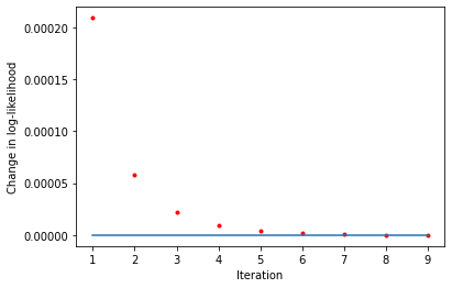
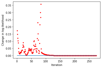
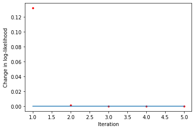
Check that log-likelihoods are monotonic
[10]:
liks1 = blm_model.liks1

print('Log-likelihoods monotonic (movers):', np.min(np.diff(liks1)) >= 0)

x_axis = range(1, len(liks1))
plt.plot(x_axis, np.diff(liks1), '.', label='liks1', color='red')
plt.plot(x_axis, np.zeros(len(liks1) - 1))
plt.xlabel('Iteration')
plt.ylabel('Change in log-likelihood')
Log-likelihoods monotonic (movers): True
[10]:
Text(0, 0.5, 'Change in log-likelihood')
[11]:
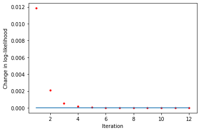
liks0 = blm_model.liks0

print('Log-likelihoods monotonic (stayers):', np.min(np.diff(liks0)) >= 0)

x_axis = range(1, len(liks0))
plt.plot(x_axis, np.diff(liks0), '.', label='liks0', color='red')
plt.plot(x_axis, np.zeros(len(liks0) - 1))
plt.xlabel('Iteration')
plt.ylabel('Change in log-likelihood')
Log-likelihoods monotonic (stayers): True
[11]:
Text(0, 0.5, 'Change in log-likelihood')
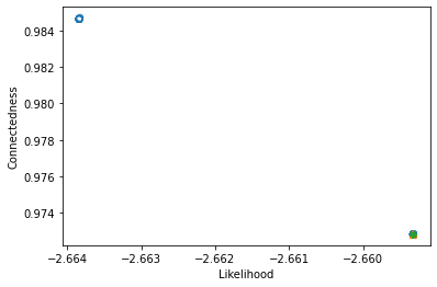
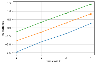
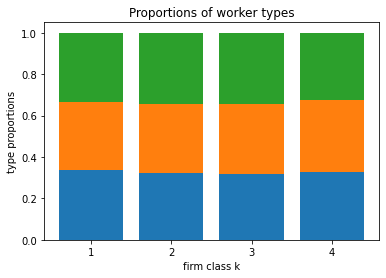
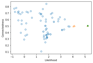
Now we can investigate the results
[12]:
# Plot likelihood vs. connectedness
blm_fit.plot_liks_connectedness()
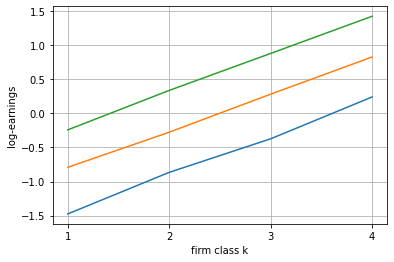
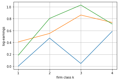
[13]:
blm_fit.plot_log_earnings()
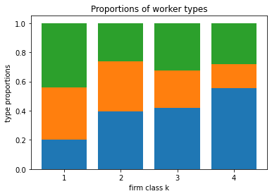
[14]:
blm_fit.plot_type_proportions()

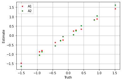
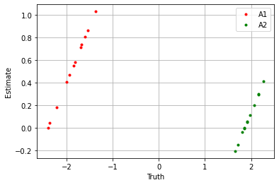
Finally, we can compare estimates to the truth
[15]:
# Compute true parameters
true_A1 = np.expand_dims(sim_data_unobserved.groupby('l1')['alpha1'].mean().to_numpy(), 1) + np.tile(sim_data_unobserved.groupby('k1')['psi1'].mean().to_numpy(), (nl, 1))
true_A2 = np.expand_dims(sim_data_unobserved.groupby('l2')['alpha2'].mean().to_numpy(), 1) + np.tile(sim_data_unobserved.groupby('k2')['psi2'].mean().to_numpy(), (nl, 1))

# Sort estimated parameters (this is because the firm type order generated by clustering is random - this is automatically handled in the built-in plotting functions)
A1, A2 = blm_model._sort_parameters(blm_model.A1, blm_model.A2, sort_firm_types=True)
[16]:
plt.plot(true_A1.flatten(), A1.flatten(), '.', label='A1', color='red')
plt.plot(true_A2.flatten(), A2.flatten(), '.', label='A2', color='green')
plt.xlabel('Truth')
plt.ylabel('Estimate')
plt.legend()
plt.grid()
plt.show()
Bootstrapped errors
The package contains the class BLMBootstrap, which allows for the construction of bootstrapped error bars.
In this example, we use the same simulated data and estimation parameters as in the previous example.
[ ]:
# Initialize BLM bootstrap estimator
blm_fit = tw.BLMBootstrap(blm_params)
# Fit BLM estimator
blm_fit.fit(
    jdata=jdata, sdata=sdata,
    blm_model=blm_model,
    n_samples=20,
    cluster_params=cluster_params,
    ncore=8,
    verbose=False
)
Now we can investigate the results
[18]:
blm_fit.plot_log_earnings()
[19]:
blm_fit.plot_type_proportions()
Control variables
Hint
Check out how to add custom columns to your BipartitePandas DataFrame here! If you don’t add custom columns properly, they may not be handled during data cleaning and estimation how you want and/or expect!
Simulating data with controls
The package contains functions to simulate data from the BLM dgp. We use this here to see how to use control variables.
In this example, we simulate a categorical, non-stationary, non-worker-type-interaction control variable. We use a low variance to ensure stability of the estimator.
Check out simulation parameter options
Do this by running:
Simulating Categorical Controls -
tw.sim_categorical_control_params().describe_all()Simulating Continuous Controls -
tw.sim_continuous_control_params().describe_all()
Alternatively, run x_params().keys() to view all the keys for a parameter dictionary, then x_params().describe(key) to get a description for a single key.
Set simulation parameter choices
[20]:
n_control = 2 # Number of types for control variable

sim_cat_params = tw.sim_categorical_control_params({
    'n': n_control,
    'stationary_A': False, 'stationary_S': False,
    'worker_type_interaction': False,
    'a1_mu': -0.5, 'a1_sig': 0.25, 'a2_mu': 0.5, 'a2_sig': 0.25,
    's1_low': 0, 's1_high': 0.01, 's2_low': 0, 's2_high': 0.01
})
sim_cts_params = tw.sim_continuous_control_params({
    'stationary_A': True, 'stationary_S': True,
    'worker_type_interaction': True,
    'a1_mu': -0.15, 'a1_sig': 0.05, 'a2_mu': 0.15, 'a2_sig': 0.05,
    's1_low': 0, 's1_high': 0.01, 's2_low': 0, 's2_high': 0.01
})
sim_blm_params = tw.sim_blm_params({
    'nl': nl, 'nk': nk,
    'a1_mu': -2, 'a1_sig': 0.25, 'a2_mu': 2, 'a2_sig': 0.25,
    's1_low': 0, 's1_high': 0.01, 's2_low': 0, 's2_high': 0.01,
    'categorical_controls': {'cat_control': sim_cat_params},
    'continuous_controls': {'cts_control': sim_cts_params}
})
Estimating control variables
PyTwoWay allows for categorical and continuous control variables.
Categorical
To define a categorical control variable, construct an instance of the parameter dictionary tw.categorical_control_params().
Then, inside an instance of blm_params(), link the key 'categorical_controls' to a dictionary linking column names to their associated parameter dictionaries.
Continuous
To define a continuous control variable, construct an instance of the parameter dictionary tw.continuous_control_params().
Then, inside an instance of blm_params(), link the key 'continuous_controls' to a dictionary linking column names to their associated parameter dictionaries.
Constraints
Constraints can be specified for control variables. They are set through the cons_a and cons_s keys for a given control variable’s parameter dictionary, except for NoWorkerTypeInteraction(). Constraint options are: - Linear() - for a fixed firm type, worker types effects must change linearly - Monotonic() - for a fixed firm type, worker types effects must increase (or decrease) monotonically - NoWorkerTypeInteraction() - for a fixed firm type, worker types effects must
all be the same - Stationary() - worker-firm pair effects are the same in all periods - StationaryFirmTypeVariation() - firm type induced variation of worker-firm pair effects is the same in all periods. In particular, this is equivalent to setting A2 = (np.mean(A2, axis=1) + A1.T - np.mean(A1, axis=1)).T. - BoundedBelow() - worker-firm pair effects are bounded below - BoundedAbove() - worker-firm pair effects are bounded above
NoWorkerTypeInteraction() is not specified through the cons_a and cons_s keys. Instead, if you want a control variable to interact with the unobserved worker types, this can be specified by setting worker_type_interaction=True in the control variable’s parameter dictionary.
Warning
Be careful when adding constraints to categorical control variables (note that not interacting with worker types requires constraints). Because categorical control variables require normalization, the choice of how to normalize can alter parameter estimates. This may raise a warning if the normalization gets stuck in a cycle of changing how to normalize every loop and the estimator is not converging. The estimator will work if you set force_min_firm_type=True in your BLM parameter dictionary
- the warning will also provide a reminder of this option.
Check out estimation parameter options
Do this by running:
Estimating Categorical Controls -
tw.categorical_control_params().describe_all()Estimating Continuous Controls -
tw.continuous_control_params().describe_all()
Alternatively, run x_params().keys() to view all the keys for a parameter dictionary, then x_params().describe(key) to get a description for a single key.
Set estimation parameter choices
[21]:
cat_params = tw.categorical_control_params({
    'n': n_control,
    'worker_type_interaction': False,
    'cons_a': None, 'cons_s': None,
    'a1_mu': -0.5, 'a1_sig': 0.25, 'a2_mu': 0.5, 'a2_sig': 0.25,
    's1_low': 0, 's1_high': 0.01, 's2_low': 0, 's2_high': 0.01
})
cts_params = tw.continuous_control_params({
    'worker_type_interaction': True,
    'cons_a': cons.Stationary(), 'cons_s': cons.Stationary(),
    'a1_mu': -0.15, 'a1_sig': 0.05, 'a2_mu': 0.15, 'a2_sig': 0.05,
    's1_low': 0, 's1_high': 0.01, 's2_low': 0, 's2_high': 0.01
})
blm_params = tw.blm_params({
    'nl': nl, 'nk': nk,
    'a1_mu': -2, 'a1_sig': 0.25, 'a2_mu': 2, 'a2_sig': 0.25,
    's1_low': 0, 's1_high': 0.01, 's2_low': 0, 's2_high': 0.01,
    'categorical_controls': {'cat_control': cat_params},
    'continuous_controls': {'cts_control': cts_params},
    'force_min_firm_type': True
})
Simulate data
sim_data gives a dictionary where the key 'jdata' gives simulated mover data and the key 'sdata' gives simulated stayer data.
sim_params gives a dictionary that links each type of control variable to the simulated parameter values for that type.
[22]:
blm_true = tw.SimBLM(sim_blm_params)
sim_data, sim_params = blm_true.simulate(return_parameters=True)
jdata, sdata = sim_data['jdata'], sim_data['sdata']
[23]:
print('Movers data')
display(jdata)
print('Stayers data')
display(sdata)
print('Simulated parameter values')
display(sim_params)
Movers data
| i | j1 | j2 | y1 | y2 | g1 | g2 | m | cat_control1 | cat_control2 | cts_control1 | cts_control2 | l | |
|---|---|---|---|---|---|---|---|---|---|---|---|---|---|
| 0 | 0 | 0 | 1 | -1.405170 | 2.884550 | 0 | 0 | 1 | 0 | 1 | -1.597127 | -0.863375 | 1 |
| 1 | 1 | 0 | 1 | -2.944559 | 2.699658 | 0 | 0 | 1 | 1 | 1 | 0.418682 | 0.439516 | 1 |
| 2 | 2 | 1 | 0 | -1.283777 | 2.810403 | 0 | 0 | 1 | 0 | 1 | -2.397280 | -0.507434 | 1 |
| 3 | 3 | 0 | 1 | -2.674142 | 2.781658 | 0 | 0 | 1 | 1 | 1 | -1.445132 | -0.133028 | 1 |
| 4 | 4 | 0 | 1 | -2.810683 | 2.110046 | 0 | 0 | 1 | 1 | 0 | -0.464561 | 1.254681 | 1 |
| ... | ... | ... | ... | ... | ... | ... | ... | ... | ... | ... | ... | ... | ... |
| 155 | 155 | 7 | 6 | -1.076676 | 1.609433 | 3 | 3 | 1 | 0 | 0 | -0.801424 | 1.277516 | 2 |
| 156 | 156 | 6 | 7 | -2.718684 | 1.932711 | 3 | 3 | 1 | 1 | 0 | 0.094787 | -0.568200 | 0 |
| 157 | 157 | 6 | 7 | -2.753058 | 1.655190 | 3 | 3 | 1 | 1 | 0 | 0.292111 | 1.155452 | 0 |
| 158 | 158 | 6 | 7 | -2.889319 | 2.357755 | 3 | 3 | 1 | 1 | 1 | 1.194183 | -0.255207 | 0 |
| 159 | 159 | 7 | 6 | -1.292902 | 2.245363 | 3 | 3 | 1 | 0 | 0 | 0.035616 | 1.193493 | 1 |
160 rows × 13 columns
Stayers data
| i | j1 | j2 | y1 | y2 | g1 | g2 | m | cat_control1 | cat_control2 | cts_control1 | cts_control2 | l | |
|---|---|---|---|---|---|---|---|---|---|---|---|---|---|
| 0 | 160 | 0 | 0 | -3.065299 | 2.939253 | 0 | 0 | 0 | 1 | 1 | 1.280102 | -1.276638 | 1 |
| 1 | 161 | 1 | 1 | -3.308012 | 1.882332 | 0 | 0 | 0 | 1 | 0 | 0.673731 | 0.978745 | 2 |
| 2 | 162 | 1 | 1 | -2.048957 | 2.500295 | 0 | 0 | 0 | 0 | 1 | 0.188291 | -0.354548 | 0 |
| 3 | 163 | 1 | 1 | -1.647712 | 3.035064 | 0 | 0 | 0 | 0 | 1 | 0.224408 | -1.773956 | 1 |
| 4 | 164 | 0 | 0 | -1.753908 | 2.028478 | 0 | 0 | 0 | 0 | 0 | -0.307819 | 0.595909 | 2 |
| 5 | 165 | 1 | 1 | -1.838391 | 3.205352 | 0 | 0 | 0 | 0 | 1 | -0.034964 | -1.680496 | 2 |
| 6 | 166 | 0 | 0 | -1.825758 | 2.394916 | 0 | 0 | 0 | 0 | 1 | -0.045699 | 0.869568 | 2 |
| 7 | 167 | 0 | 0 | -3.162265 | 3.055979 | 0 | 0 | 0 | 1 | 1 | 0.174373 | -1.324212 | 2 |
| 8 | 168 | 0 | 0 | -2.035432 | 2.368199 | 0 | 0 | 0 | 0 | 1 | 0.227607 | 0.600801 | 0 |
| 9 | 169 | 0 | 0 | -2.933966 | 2.556052 | 0 | 0 | 0 | 1 | 1 | 0.343777 | 1.315978 | 1 |
| 10 | 170 | 2 | 2 | -1.441650 | 2.437222 | 1 | 1 | 0 | 0 | 1 | -0.352137 | -0.029504 | 1 |
| 11 | 171 | 3 | 3 | -1.681946 | 2.603666 | 1 | 1 | 0 | 0 | 1 | 0.797169 | -0.100233 | 0 |
| 12 | 172 | 3 | 3 | -1.446450 | 2.115750 | 1 | 1 | 0 | 0 | 0 | -0.856424 | -0.023039 | 0 |
| 13 | 173 | 3 | 3 | -3.140376 | 2.507038 | 1 | 1 | 0 | 1 | 1 | 2.209182 | 0.660209 | 0 |
| 14 | 174 | 2 | 2 | -2.743617 | 2.046139 | 1 | 1 | 0 | 1 | 0 | 0.038795 | -0.846242 | 1 |
| 15 | 175 | 3 | 3 | -1.253390 | 1.997722 | 1 | 1 | 0 | 0 | 0 | -1.620871 | -0.369944 | 1 |
| 16 | 176 | 3 | 3 | -2.042038 | 1.745926 | 1 | 1 | 0 | 1 | 0 | -1.510300 | 0.903805 | 2 |
| 17 | 177 | 3 | 3 | -1.678088 | 2.148858 | 1 | 1 | 0 | 0 | 0 | 0.876064 | -0.305209 | 0 |
| 18 | 178 | 2 | 2 | -1.539851 | 2.806150 | 1 | 1 | 0 | 0 | 1 | -0.193820 | -1.547240 | 0 |
| 19 | 179 | 2 | 2 | -1.484411 | 2.540243 | 1 | 1 | 0 | 0 | 1 | 0.029680 | -0.694832 | 1 |
| 20 | 180 | 5 | 5 | -1.145073 | 1.938436 | 2 | 2 | 0 | 0 | 1 | 0.448419 | 1.062856 | 2 |
| 21 | 181 | 5 | 5 | -1.976578 | 2.167116 | 2 | 2 | 0 | 0 | 0 | 0.051553 | 0.623657 | 0 |
| 22 | 182 | 5 | 5 | -2.248826 | 2.782804 | 2 | 2 | 0 | 1 | 1 | -0.069256 | -1.654039 | 2 |
| 23 | 183 | 4 | 4 | -3.381418 | 2.342920 | 2 | 2 | 0 | 1 | 0 | 0.835689 | -0.528370 | 0 |
| 24 | 184 | 5 | 5 | -2.414065 | 1.897629 | 2 | 2 | 0 | 1 | 0 | -0.123666 | 0.956612 | 1 |
| 25 | 185 | 4 | 4 | -3.131777 | 2.884738 | 2 | 2 | 0 | 1 | 1 | -0.767185 | -0.904343 | 0 |
| 26 | 186 | 4 | 4 | -3.342341 | 2.693796 | 2 | 2 | 0 | 1 | 1 | 0.726720 | 0.368079 | 0 |
| 27 | 187 | 5 | 5 | -2.140324 | 2.530651 | 2 | 2 | 0 | 0 | 0 | 1.183305 | -1.663274 | 0 |
| 28 | 188 | 4 | 4 | -3.219936 | 2.662715 | 2 | 2 | 0 | 1 | 1 | -0.267946 | 0.635036 | 0 |
| 29 | 189 | 4 | 4 | -2.813351 | 2.204771 | 2 | 2 | 0 | 1 | 0 | 1.858780 | -1.423794 | 2 |
| 30 | 190 | 6 | 6 | -2.627046 | 2.341005 | 3 | 3 | 0 | 1 | 1 | -0.732658 | -0.174954 | 0 |
| 31 | 191 | 7 | 7 | -1.475745 | 1.854227 | 3 | 3 | 0 | 0 | 0 | 0.085931 | -0.259650 | 0 |
| 32 | 192 | 7 | 7 | -1.372760 | 1.618090 | 3 | 3 | 0 | 0 | 0 | 0.247395 | 1.038758 | 2 |
| 33 | 193 | 6 | 6 | -1.396256 | 1.879039 | 3 | 3 | 0 | 0 | 0 | -0.298457 | -0.415220 | 0 |
| 34 | 194 | 6 | 6 | -1.349778 | 2.194202 | 3 | 3 | 0 | 0 | 1 | -0.641476 | 0.840362 | 0 |
| 35 | 195 | 7 | 7 | -1.435867 | 1.505834 | 3 | 3 | 0 | 0 | 0 | 0.455100 | 1.541480 | 2 |
| 36 | 196 | 6 | 6 | -2.786497 | 1.745557 | 3 | 3 | 0 | 1 | 0 | 0.631748 | 0.769990 | 0 |
| 37 | 197 | 7 | 7 | -1.450763 | 1.851792 | 3 | 3 | 0 | 0 | 0 | -0.047915 | -0.048053 | 0 |
| 38 | 198 | 6 | 6 | -2.567547 | 1.749243 | 3 | 3 | 0 | 1 | 0 | -0.018666 | 0.676466 | 2 |
| 39 | 199 | 7 | 7 | -2.342840 | 2.728105 | 3 | 3 | 0 | 1 | 1 | -1.548878 | 1.056820 | 1 |
Simulated parameter values
{'A1': array([[-2.40434291, -1.93230882, -2.3641309 , -1.81931006],
        [-1.99649895, -1.8539811 , -1.54271365, -1.67049293],
        [-2.21882556, -1.59916272, -1.37328134, -1.69013257]]),
 'A2': array([[1.85490342, 1.97296398, 2.15268324, 1.7112059 ],
        [2.15476764, 1.81388297, 1.90973225, 2.26752212],
        [2.0604013 , 1.90970787, 1.65698835, 1.84848259]]),
 'S1': array([[6.24733520e-03, 3.25013934e-04, 9.95248435e-03, 7.88841644e-03],
        [5.06607130e-04, 5.60070089e-05, 5.12086700e-03, 8.94274499e-03],
        [1.15689335e-03, 3.52890499e-03, 3.17502080e-03, 9.56078356e-03]]),
 'S2': array([[0.00106304, 0.00627278, 0.0096796 , 0.00626775],
        [0.00905057, 0.00542163, 0.00412828, 0.00967574],
        [0.00684023, 0.00786226, 0.00925993, 0.00867167]]),
 'pk1': array([[0.22439344, 0.64001715, 0.13558941],
        [0.30791439, 0.16101403, 0.53107158],
        [0.13470115, 0.14758551, 0.71771334],
        [0.15657995, 0.31968694, 0.5237331 ],
        [0.08722402, 0.82393394, 0.08884205],
        [0.81811766, 0.03811832, 0.14376401],
        [0.13887305, 0.03062248, 0.83050447],
        [0.44799947, 0.31514629, 0.23685424],
        [0.42634457, 0.25005179, 0.32360364],
        [0.41872874, 0.15005459, 0.43121667],
        [0.36605   , 0.26067997, 0.37327004],
        [0.38861717, 0.46752657, 0.14385626],
        [0.81362141, 0.10810991, 0.07826868],
        [0.66945685, 0.10447555, 0.2260676 ],
        [0.29082898, 0.26732746, 0.44184356],
        [0.28325089, 0.55597618, 0.16077293]]),
 'pk0': array([[0.14716973, 0.33066942, 0.52216085],
        [0.6236124 , 0.33471458, 0.04167301],
        [0.34365961, 0.23123918, 0.42510121],
        [0.71334724, 0.06543533, 0.22121742]]),
 'A1_cat': {'cat_control': array([ 0.37500106, -0.88596277])},
 'A2_cat': {'cat_control': array([0.12246111, 0.60852562])},
 'S1_cat': {'cat_control': array([0.00785542, 0.00410917])},
 'S2_cat': {'cat_control': array([0.00749964, 0.00787043])},
 'A1_cts': {'cts_control': array([-0.14213511, -0.14125649, -0.30366185])},
 'A2_cts': {'cts_control': array([-0.14213511, -0.14125649, -0.30366185])},
 'S1_cts': {'cts_control': array([0.00774112, 0.00157575, 0.00477038])},
 'S2_cts': {'cts_control': array([0.00774112, 0.00157575, 0.00477038])}}
Initialize and run BLMEstimator
[ ]:
# Initialize BLM estimator
blm_fit = tw.BLMEstimator(blm_params)
# Fit BLM estimator
blm_fit.fit(jdata=jdata, sdata=sdata, n_init=80, n_best=5, ncore=8)
# Store best model
blm_model = blm_fit.model
Check that log-likelihoods are monotonic
[25]:
liks1 = blm_model.liks1[1:]

print('Log-likelihoods monotonic (movers):', np.min(np.diff(liks1)) >= 0)

x_axis = range(1, len(liks1))
plt.plot(x_axis, np.diff(liks1), '.', label='liks1', color='red')
plt.plot(x_axis, np.zeros(len(liks1) - 1))
plt.xlabel('Iteration')
plt.ylabel('Change in log-likelihood')
Log-likelihoods monotonic (movers): True
[25]:
Text(0, 0.5, 'Change in log-likelihood')
[26]:
liks0 = blm_model.liks0

print('Log-likelihoods monotonic (stayers):', np.min(np.diff(liks0)) >= 0)

x_axis = range(1, len(liks0))
plt.plot(x_axis, np.diff(liks0), '.', label='liks0', color='red')
plt.plot(x_axis, np.zeros(len(liks0) - 1))
plt.xlabel('Iteration')
plt.ylabel('Change in log-likelihood')
Log-likelihoods monotonic (stayers): True
[26]:
Text(0, 0.5, 'Change in log-likelihood')
Now we can investigate the results
[27]:
# Plot likelihood vs. connectedness
blm_fit.plot_liks_connectedness()
[28]:
blm_fit.plot_log_earnings()
[29]:
blm_fit.plot_type_proportions()
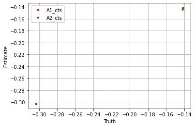
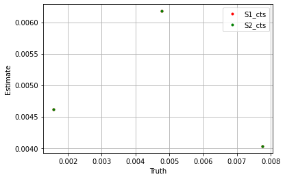
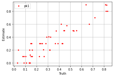
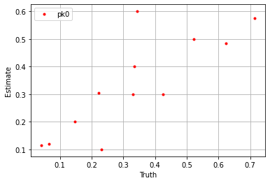
Finally, we can compare estimates to the truth
[30]:
plt.plot(sim_params['A1'].flatten(), blm_model.A1.flatten(), '.', label='A1', color='red')
plt.plot(sim_params['A2'].flatten(), blm_model.A2.flatten(), '.', label='A2', color='green')
plt.xlabel('Truth')
plt.ylabel('Estimate')
plt.legend()
plt.grid()
plt.show()
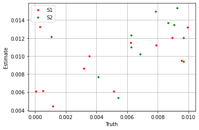
plt.plot(sim_params['S1'].flatten(), blm_model.S1.flatten(), '.', label='S1', color='red')
plt.plot(sim_params['S2'].flatten(), blm_model.S2.flatten(), '.', label='S2', color='green')
plt.xlabel('Truth')
plt.ylabel('Estimate')
plt.legend()
plt.grid()
plt.show()
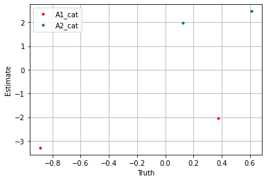
plt.plot(sim_params['A1_cat']['cat_control'].flatten(), blm_model.A1_cat['cat_control'].flatten(), '.', label='A1_cat', color='red')
plt.plot(sim_params['A2_cat']['cat_control'].flatten(), blm_model.A2_cat['cat_control'].flatten(), '.', label='A2_cat', color='green')
plt.xlabel('Truth')
plt.ylabel('Estimate')
plt.legend()
plt.grid()
plt.show()
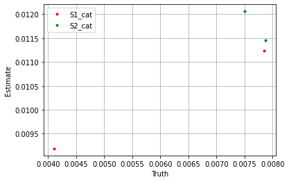
plt.plot(sim_params['S1_cat']['cat_control'].flatten(), blm_model.S1_cat['cat_control'].flatten(), '.', label='S1_cat', color='red')
plt.plot(sim_params['S2_cat']['cat_control'].flatten(), blm_model.S2_cat['cat_control'].flatten(), '.', label='S2_cat', color='green')
plt.xlabel('Truth')
plt.ylabel('Estimate')
plt.legend()
plt.grid()
plt.show()
plt.plot(sim_params['A1_cts']['cts_control'].flatten(), blm_model.A1_cts['cts_control'].flatten(), '.', label='A1_cts', color='red')
plt.plot(sim_params['A2_cts']['cts_control'].flatten(), blm_model.A2_cts['cts_control'].flatten(), '.', label='A2_cts', color='green')
plt.xlabel('Truth')
plt.ylabel('Estimate')
plt.legend()
plt.grid()
plt.show()
plt.plot(sim_params['S1_cts']['cts_control'].flatten(), blm_model.S1_cts['cts_control'].flatten(), '.', label='S1_cts', color='red')
plt.plot(sim_params['S2_cts']['cts_control'].flatten(), blm_model.S2_cts['cts_control'].flatten(), '.', label='S2_cts', color='green')
plt.xlabel('Truth')
plt.ylabel('Estimate')
plt.legend()
plt.grid()
plt.show()
plt.plot(sim_params['pk1'].flatten(), blm_model.pk1.flatten(), '.', label='pk1', color='red')
plt.xlabel('Truth')
plt.ylabel('Estimate')
plt.legend()
plt.grid()
plt.show()
plt.plot(sim_params['pk0'].flatten(), blm_model.pk0.flatten(), '.', label='pk0', color='red')
plt.xlabel('Truth')
plt.ylabel('Estimate')
plt.legend()
plt.grid()
plt.show()
Warning
The parameters are identified only up to a constant intercept.
Because of this, to maintain consistency between estimations, PyTwoWay automatically normalizes worker-firm types to have effect 0, depending on the control variables used (normalization only occurs with categorical control variables - for a stationary control variable, only the first period is normalized (if it is non-stationary, both periods are normalized); for a control variable that does not interact with worker types, only the lowest worker type is normalized (if it does interact with worker types, all worker types are normalized)).
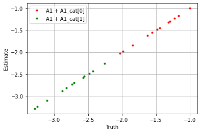
If we take the sum over the estimators we see the model performs well.
[31]:
## First period ##
plt.plot(
(sim_params['A1'] + sim_params['A1_cat']['cat_control'][0]).flatten(),
(blm_model.A1 + blm_model.A1_cat['cat_control'][0]).flatten(),
'.', label='A1 + A1_cat[0]', color='red'
)
plt.plot(
(sim_params['A1'] + sim_params['A1_cat']['cat_control'][1]).flatten(),
(blm_model.A1 + blm_model.A1_cat['cat_control'][1]).flatten(),
'.', label='A1 + A1_cat[1]', color='green'
)
plt.xlabel('Truth')
plt.ylabel('Estimate')
plt.legend()
plt.grid()
plt.show()
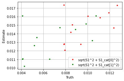
plt.plot(
np.sqrt((sim_params['S1'] ** 2 + sim_params['S1_cat']['cat_control'][0] ** 2).flatten()),
np.sqrt((blm_model.S1 ** 2 + blm_model.S1_cat['cat_control'][0] ** 2).flatten()),
'.', label='sqrt(S1^2 + S1_cat[0]^2)', color='red'
)
plt.plot(
np.sqrt((sim_params['S1'] ** 2 + sim_params['S1_cat']['cat_control'][1] ** 2).flatten()),
np.sqrt((blm_model.S1 ** 2 + blm_model.S1_cat['cat_control'][1] ** 2).flatten()),
'.', label='sqrt(S1^2 + S1_cat[1]^2)', color='green'
)
plt.xlabel('Truth')
plt.ylabel('Estimate')
plt.legend()
plt.grid()
plt.show()
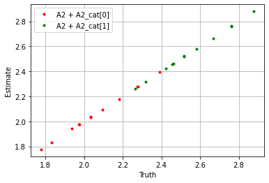
## Second period ##
plt.plot(
(sim_params['A2'] + sim_params['A2_cat']['cat_control'][0]).flatten(),
(blm_model.A2 + blm_model.A2_cat['cat_control'][0]).flatten(),
'.', label='A2 + A2_cat[0]', color='red'
)
plt.plot(
(sim_params['A2'] + sim_params['A2_cat']['cat_control'][1]).flatten(),
(blm_model.A2 + blm_model.A2_cat['cat_control'][1]).flatten(),
'.', label='A2 + A2_cat[1]', color='green'
)
plt.xlabel('Truth')
plt.ylabel('Estimate')
plt.legend()
plt.grid()
plt.show()
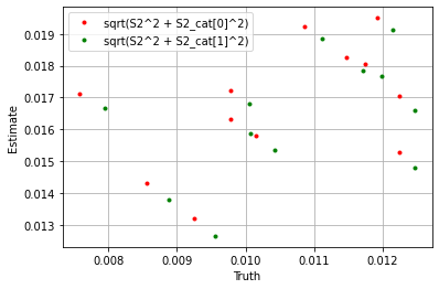
plt.plot(
np.sqrt((sim_params['S2'] ** 2 + sim_params['S2_cat']['cat_control'][0] ** 2).flatten()),
np.sqrt((blm_model.S2 ** 2 + blm_model.S2_cat['cat_control'][0] ** 2).flatten()),
'.', label='sqrt(S2^2 + S2_cat[0]^2)', color='red'
)
plt.plot(
np.sqrt((sim_params['S2'] ** 2 + sim_params['S2_cat']['cat_control'][1] ** 2).flatten()),
np.sqrt((blm_model.S2 ** 2 + blm_model.S2_cat['cat_control'][1] ** 2).flatten()),
'.', label='sqrt(S2^2 + S2_cat[1]^2)', color='green'
)
plt.xlabel('Truth')
plt.ylabel('Estimate')
plt.legend()
plt.grid()
plt.show()
Variance decomposition
The package contains the class BLMVarianceDecomposition, which allows for the estimation of the decomposition of the variance components of the BLM estimator.
In this example, we use the same simulated data and estimation parameters as in the previous example.
[ ]:
# Initialize BLM variance decomposition estimator
blm_fit = tw.BLMVarianceDecomposition(blm_params)
# Fit BLM estimator
blm_fit.fit(
    jdata=jdata, sdata=sdata,
    blm_model=blm_model,
    n_samples=20,
    Q_var=[
        tw.Q.VarCovariate('psi'),
        tw.Q.VarCovariate('cat_control'),
        tw.Q.VarCovariate('cts_control')
    ],
    ncore=1
)
Investigate the results
Results correspond to:
y: income (outcome) columneps: residualpsi: firm effectsalpha: worker effects
Note
Results from all estimations are stored in the class attribute dictionary .res. We take the mean, but storing all results gives the option to estimate different sample statistics.
Note
The particular variance that is estimated is controlled through the parameter 'Q_var' and the covariance that is estimated is controlled through the parameter 'Q_cov'.
By default, the variance is var(psi) and the covariance is cov(psi, alpha). The default estimates don’t include var(alpha), but if you don’t include controls, var(alpha) can be computed as the residual from var(y) = var(psi) + var(alpha) + 2 * cov(psi, alpha) + var(eps).
[33]:
for k, v in blm_fit.res.items():
    print(f'{k!r}: {v.mean()}')
'var(y)': 4.1784778224072054
'var(eps)': 3.862767039874967
'var(cat_control)': 0.17504851379038694
'var(cts_control)': 0.03529768004099764
'var(psi)': 0.052474105201016495
'cov(psi, alpha)': -0.0014679055738114212