Attrition example
[1]:
# Add PyTwoWay to system path (do not run this)
# import sys
# sys.path.append('../../..')
Import the PyTwoWay package
Make sure to install it using pip install pytwoway.
[2]:
import pytwoway as tw
import bipartitepandas as bpd
First, check out parameter options
Do this by running:
FE -
tw.fe_params().describe_all()CRE -
tw.cre_params().describe_all()Clustering -
bpd.cluster_params().describe_all()Cleaning -
bpd.clean_params().describe_all()Simulating -
bpd.sim_params().describe_all()
Alternatively, run x_params().keys() to view all the keys for a parameter dictionary, then x_params().describe(key) to get a description for a single key.
Second, set parameter choices
Note that we set copy=False in clean_params to avoid unnecessary copies (although this will modify the original dataframe).
[3]:
# FE
fe_params = tw.fe_params(
    {
        'ndraw_trace_ho': 10,
        'ndraw_trace_he': 20
    }
)
# Cleaning
clean_params = bpd.clean_params(
    {
        'connectedness': None,
        'drop_returns': 'returners',
        'copy': False
    }
)
# Simulating
sim_params = bpd.sim_params(
    {
        'n_workers': 8000,
        'firm_size': 20,
        'alpha_sig': 2, 'w_sig': 2,
        'c_sort': 1.5, 'c_netw': 1.5,
        'p_move': 0.2
    }
)
Third, extract data (we simulate for the example)
BipartitePandas contains the class SimBipartite which we use here to simulate a bipartite network. If you have your own data, you can import it during this step. Load it as a Pandas DataFrame and then convert it into a BipartitePandas DataFrame in the next step.
[4]:
sim_data = bpd.SimBipartite(sim_params).simulate()[['i', 'j', 'y', 't']]
Fourth, prepare data
This is exactly how you should prepare real data prior to running the FE estimator.
First, we convert the data into a
BipartitePandas DataFrameSecond, we clean the data (e.g. drop NaN observations, make sure firm and worker ids are contiguous, etc.)
Third, we collapse the data at the worker-firm spell level (taking mean wage over the spell)
Further details on BipartitePandas can be found in the package documentation, available here.
Note
For Attrition, it is recommended to initially clean the data WITHOUT taking the connected or leave-one-out set, as these will be computed during estimation, and computing either beforehand may alter estimation results.
[5]:
# Convert into BipartitePandas DataFrame
bdf = bpd.BipartiteDataFrame(sim_data)
# Clean and collapse
bdf = bdf.clean(clean_params).collapse(
    level='spell',
    is_sorted=True,
    copy=False
)
checking required columns and datatypes
sorting rows
dropping NaN observations
generating 'm' column
keeping highest paying job for i-t (worker-year) duplicates (how='max')
dropping workers who leave a firm then return to it (how='returners')
making 'i' ids contiguous
making 'j' ids contiguous
computing largest connected set (how=None)
sorting columns
resetting index
Fifth, initialize and run the estimator
[ ]:
# Initialize Attrition estimator
tw_attrition = tw.Attrition(fe_params=fe_params, estimate_bs=True)
# Fit Attrition estimator
tw_attrition.attrition(bdf, N=50, ncore=8)
Finally, generate attrition plots and boxplots
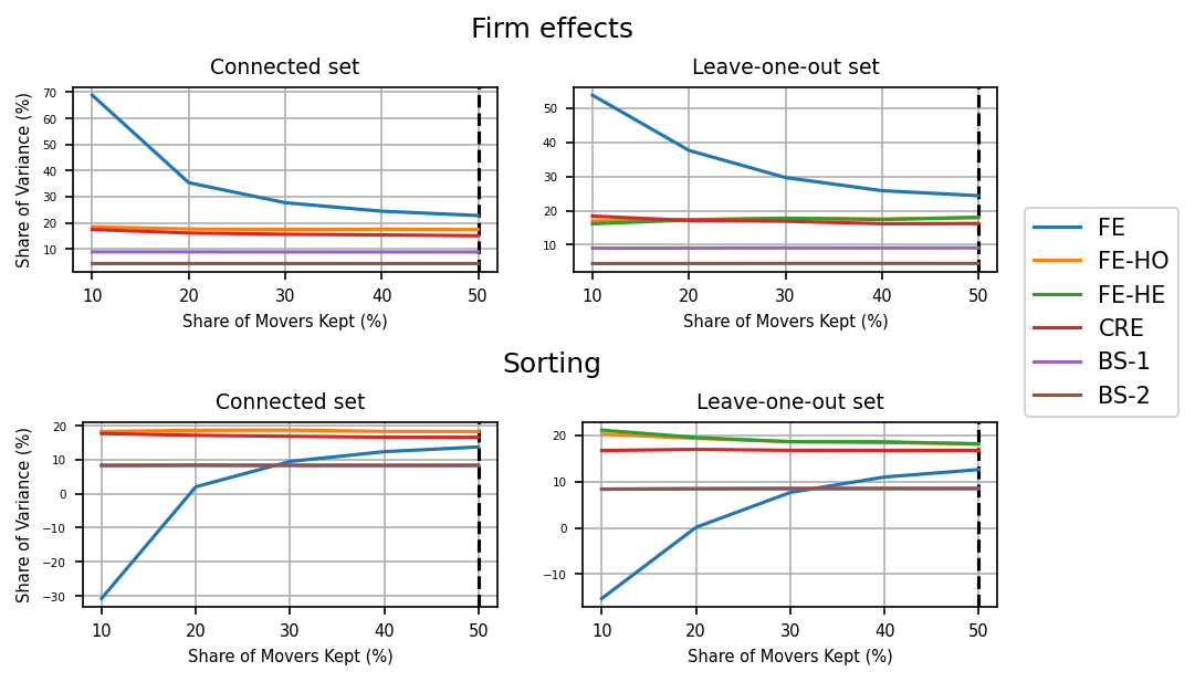
[7]:
# Plots
tw_attrition.plots()
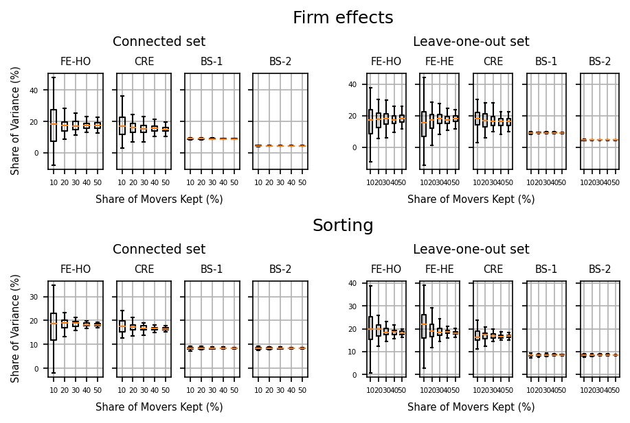
[8]:
# Boxplots
tw_attrition.boxplots()
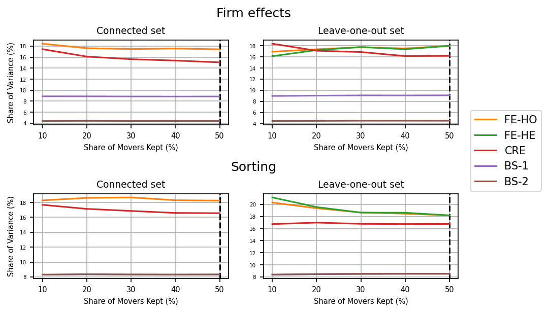
Now let’s zoom in on the bias-corrected results:
[9]:
# Plots
tw_attrition.plots(fe=False)
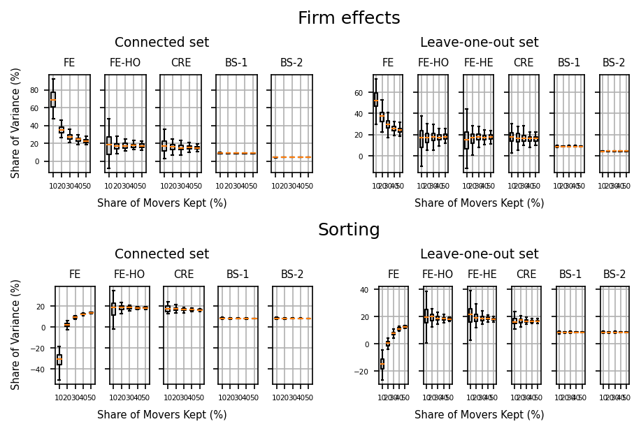
[10]:
# Boxplots
tw_attrition.boxplots(fe=False)