Hello, this is a notebook associated with the JEP article on the ABC of AKM. We provide simple simulation examples to make concrete the different points developed in the paper.

The first part is a quick dive in, while later sections go behind the scenes, explaining how the data is generated and digging deeper into the analysis.

The notebook is fully self-contained and you can look directly at all the code. Some of it is a bit lengthy so the code cell is closed to start with.

We hope this is useful and please provide any feedback directly to us.

Quick dive, simulate and estimate AKM

We start with a quick dive, brushing over the details. We use the provided functions to create a parameter set and simulate a matched data set.

np.random.seed(6344) # fixing the random seed

# initialize the model — parameters calibrated to match Guvenen/Song (US) AKM decomposition
model = Model(lambda1=0.559, rho=0.351, sigma=0.369, ng=10, nj=100,
              scale_alpha=0.550, scale_psi=0.317)

# simulate data from the model, impose connectedness
data = model.simulate(1_000, 5, connected=True)

data

Largest connected component: 100

	i	j	t	alpha	psi	epsilon	y
0	0	0	0	1.022779	0.737452	-0.309417	1.450815
1	0	0	1	1.022779	0.737452	0.243430	2.003662
2	0	1	2	1.022779	0.011801	-0.097350	0.937230
3	0	2	3	1.022779	-0.051351	0.083707	1.055135
4	0	2	4	1.022779	-0.051351	0.253446	1.224874
...	...	...	...	...	...	...	...
4995	999	25	0	-0.815266	-0.280423	-0.024718	-1.120407
4996	999	25	1	-0.815266	-0.280423	-0.241333	-1.337022
4997	999	25	2	-0.815266	-0.280423	0.118842	-0.976848
4998	999	25	3	-0.815266	-0.280423	-0.523191	-1.618881
4999	999	25	4	-0.815266	-0.280423	-0.293521	-1.389210

5000 rows × 7 columns

The data is a panel of workers with the following columns:

i: worker identifier
j: firm identifier
t: time period
alpha: worker wage fixed heterogeneity
psi: firm wage fixed heterogeneity
epsilon: wage residual
y: realized wage

True variance decomposition

There aren’t any estimates at this point. These are the true parameter values and residual realizations. We can compute the “true” variance decomposition.

# let's compute the variance decompostion and display it as a table
var_decomposition_true = variance_decomposition(data)
display_variance_decomposition(var_decomposition_true, text="True model decomposition")

True model decomposition

\(Var(\alpha)\)	\(Var(\psi)\)	\(2Cov(\alpha,\psi)\)	\(Var(\epsilon)\)
0.49	0.08	0.09	0.14
61.7%	9.6%	11.6%	17.0%

Compute AKM estimates

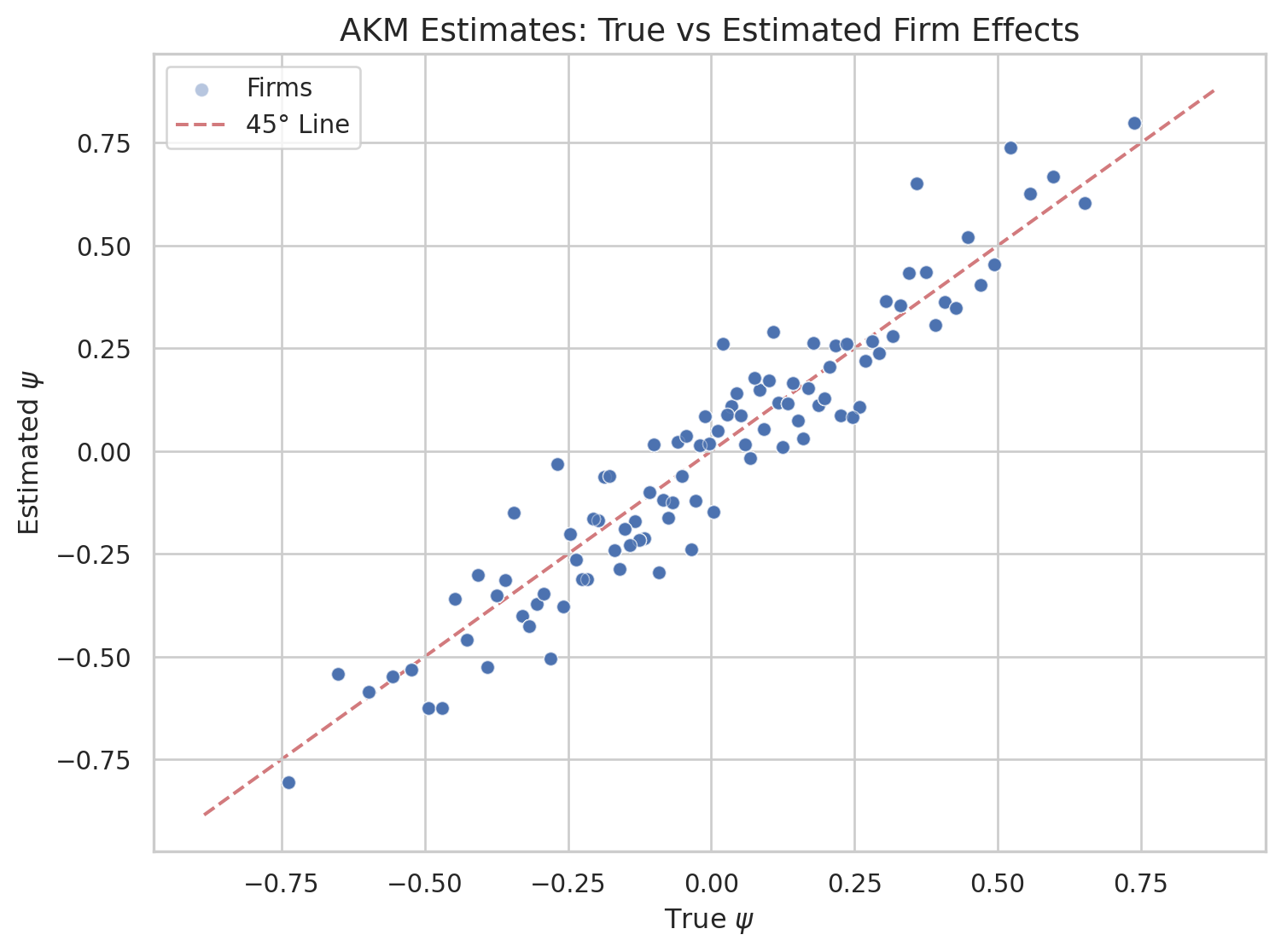
We can use the data, the columns i, j and y to compute the AKM estimates of \(\psi\) and \(\alpha\) and construct a decomposition using these estimates. When calling compute_akm, the estimated fixed effects are appended to the data in alpha_hat and psi_hat. We can plot the estimated \(\psi\) versus the true \(\psi\).

data = compute_akm(data)

# demean estimated firm effects (mean level is not identified)
data['psi_hat'] = data['psi_hat'] - data['psi_hat'].mean()

sns.set_theme(style="whitegrid")
plt.figure(figsize=(8, 6))

# Main scatter plot
plt.scatter(
    data['psi'],
    data['psi_hat'],
    alpha=0.4,
    edgecolors='w',
    linewidth=0.5,
    label='Firms'
)

# 45-degree reference line
lims = [
    np.min([plt.xlim(), plt.ylim()]),
    np.max([plt.xlim(), plt.ylim()])
]
plt.plot(lims, lims, 'r--', alpha=0.75, zorder=0, label='45° Line')

plt.xlabel(r'True $\psi$', fontsize=12)
plt.ylabel(r'Estimated $\psi$', fontsize=12)
plt.title('AKM Estimates: True vs Estimated Firm Effects', fontsize=14)
plt.legend()
plt.tight_layout()
plt.show()

Use AKM estimate to construct variance decomposition

var_decomposition_hat = variance_decomposition(data, alpha_col="alpha_hat", psi_col="psi_hat", y_col="y")
display_variance_decomposition(var_decomposition_hat, text="Estimated model decomposition")

Estimated model decomposition

\(Var(\alpha)\)	\(Var(\psi)\)	\(2Cov(\alpha,\psi)\)	\(Var(\epsilon)\)
0.51	0.09	0.08	0.10
65.5%	11.6%	9.7%	13.2%

As we can see, while we simulated from a model which satisfies all the assumptions of AKM, the realized estimated decomposition is quite off. The variance of the firm effect is much larger and the covariance is much smaller, actually slightly negative.

Monte-Carlo

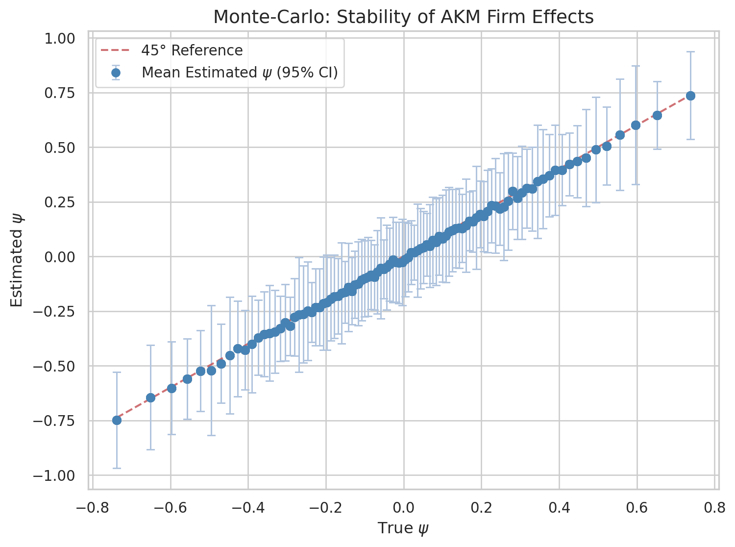
We can simulate running the estimator on randomly drawn datasets to learn whether this was only due to the seed we used and this particular draw of the residuals.

We redraw the residuals, recompute the AKM estimates, and compare the average estimate to the true estimate. Because of the properties of OLS we expect this to be very well behaved in expectation.

reps = []
var_psi_reps = []
for rep in range(100):
    psi_hat_rep = compute_akm(model.draw_residuals(data))['psi_hat']
    psi_hat_rep = psi_hat_rep - psi_hat_rep.mean()
    reps.append(psi_hat_rep)
    var_psi_reps.append(psi_hat_rep.var())
psi_hat_mean = np.vstack(reps).mean(axis=0)
psi_hat_sd = np.vstack(reps).std(axis=0)

sns.set_theme(style="whitegrid")
plt.figure(figsize=(8, 6))

# Error bar plot
plt.errorbar(data['psi'], psi_hat_mean, yerr=1.96 * psi_hat_sd,
             fmt='o', color='steelblue', ecolor='lightsteelblue',
             capsize=3, elinewidth=1, markeredgewidth=1,
             label=r'Mean Estimated $\psi$ (95% CI)')

# 45-degree reference line
lims = [np.min(data['psi']), np.max(data['psi'])]
plt.plot(lims, lims, 'r--', alpha=0.8, label='45° Reference')

plt.xlabel(r'True $\psi$', fontsize=12)
plt.ylabel(r'Estimated $\psi$', fontsize=12)
plt.title('Monte-Carlo: Stability of AKM Firm Effects', fontsize=14)
plt.legend()
plt.tight_layout()
plt.show()

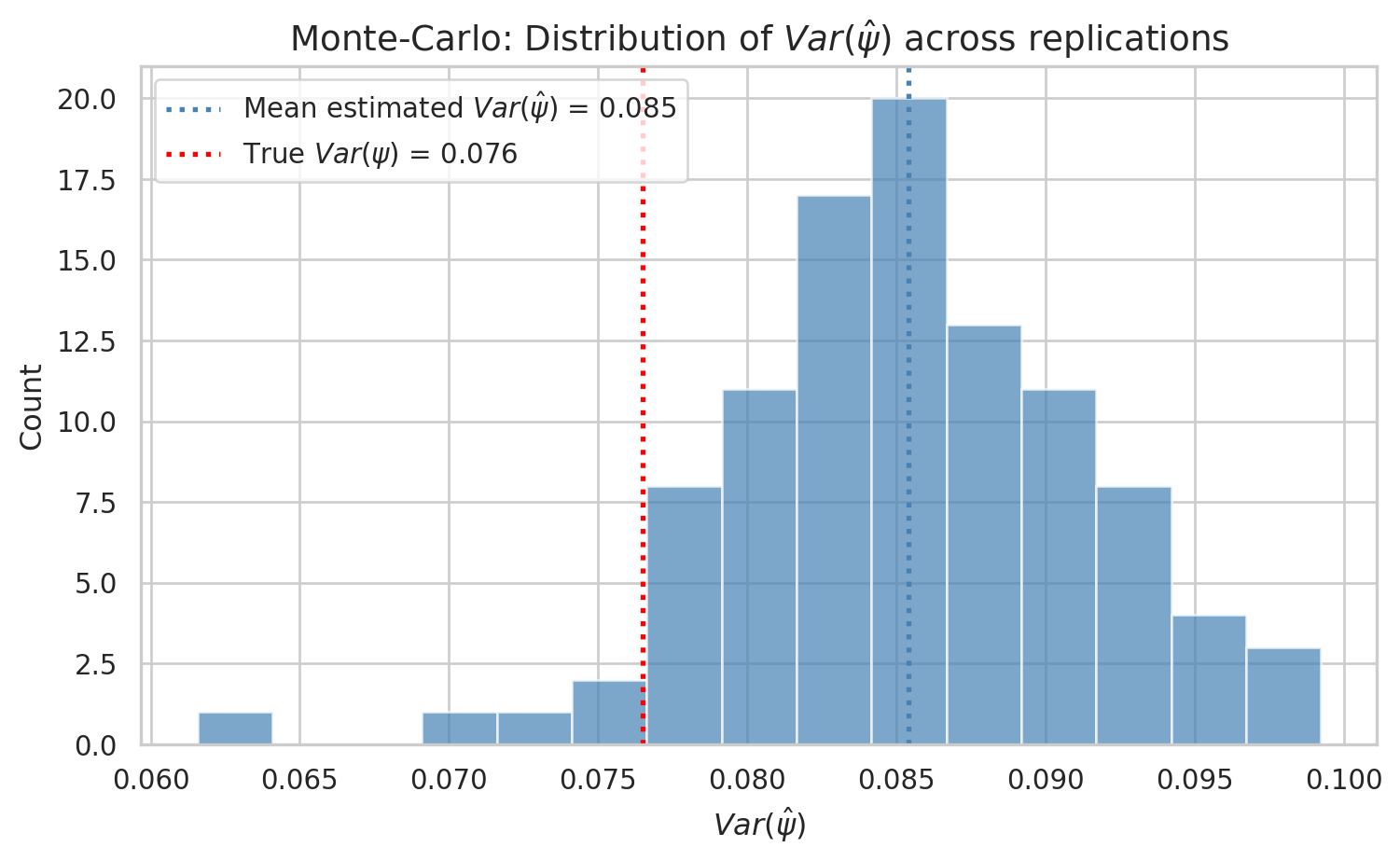
sns.set_theme(style="whitegrid")
plt.figure(figsize=(8, 5))

plt.hist(var_psi_reps, bins=15, edgecolor='white', alpha=0.7, color='steelblue')
plt.axvline(np.mean(var_psi_reps), linestyle=':', color='steelblue', linewidth=2,
            label=rf'Mean estimated $Var(\hat\psi)$ = {np.mean(var_psi_reps):.3f}')
plt.axvline(data['psi'].var(), linestyle=':', color='red', linewidth=2,
            label=rf'True $Var(\psi)$ = {data["psi"].var():.3f}')

plt.xlabel(r'$Var(\hat\psi)$', fontsize=12)
plt.ylabel('Count', fontsize=12)
plt.title(r'Monte-Carlo: Distribution of $Var(\hat\psi)$ across replications', fontsize=14)
plt.legend()
plt.tight_layout()
plt.show()

We see in the previous graph that the \(\psi\) line up very well with the true ones on average. However there is a lot of variation around the estimated values. Such variation contributes to the estimated variance.

How did we simulate the data?

The data generating process has two ingredients: a mobility model that determines how workers move across firms, and a wage equation that determines earnings. We describe each in turn, and then illustrate with a small example.

Mobility with homophily

Workers belong to one of \(n_g\) groups indexed by \(g\). Each group has a type \(\alpha_g = s_\alpha \cdot \tilde\alpha_g\) where \(\tilde\alpha_g\) is drawn from equally spaced quantiles of a standard normal and \(s_\alpha\) is a scale parameter. Firms are indexed by \(j\) and have a permanent characteristic \(\psi_j = s_\psi \cdot \tilde\psi_j\) (similarly scaled).

Each period, a worker of group \(g\) currently at firm \(j\) draws a potential alternative firm \(j'\) uniformly at random. The worker moves to \(j'\) with probability

\[ P(\text{move to } j' \mid g, j) = \frac{\lambda}{1 + \exp\!\Big(\frac{1}{\rho}\big[(\psi_{j'} - \alpha_g)^2 - (\psi_j - \alpha_g)^2\big]\Big)} \]

The key term is the difference in squared distances \((\psi_{j'} - \alpha_g)^2 - (\psi_j - \alpha_g)^2\). Workers prefer firms whose \(\psi_j\) is close to their group type \(\alpha_g\) — this is the homophily (or sorting) in the model. The parameter \(\rho\) controls sensitivity: large \(\rho\) means workers care little about match quality and move frequently; small \(\rho\) means workers are very selective. The parameter \(\lambda\) scales the overall mobility rate.

At \(t=0\), each worker’s initial firm is drawn from the stationary distribution of the Markov chain implied by this transition rule.

Wage equation

Wages follow the standard AKM additive structure:

\[ y_{it} = \alpha_i + \psi_{j(i,t)} + \epsilon_{it}, \qquad \epsilon_{it} \sim \mathcal{N}(0, \sigma^2) \]

The individual effect \(\alpha_i\) is drawn as \(\alpha_i = \alpha_g + u_i\) where \(u_i \sim \mathcal{N}(0, s_\alpha^2)\), so workers in the same group share a common component but differ idiosyncratically. The firm effect \(\psi_{j}\) in the wage equation is the same \(\psi_j\) that governs mobility, which ensures that the sorting pattern in mobility directly creates a correlation between \(\alpha_i\) and \(\psi_j\) in the wage data.

Summary of parameters

The simulation is controlled by the following parameters:

Parameter	Description
\(\lambda\) (`lambda1`)	Mobility rate — scales the probability of moving to a new firm each period. Higher values produce more job-to-job transitions.
\(\rho\) (`rho`)	Sorting temperature — controls how sensitive mobility is to match quality. Large \(\rho\) weakens sorting (workers move nearly at random); small \(\rho\) strengthens it (workers only move to better-matched firms).
\(\sigma\) (`sigma`)	Wage noise — standard deviation of the i.i.d. residual \(\epsilon_{it}\). Larger values make wages noisier relative to the fixed effects.
\(s_\alpha\) (`scale_alpha`)	Worker-effect scale — multiplies both the group component \(\tilde\alpha_g\) and the idiosyncratic draw \(u_i\). Controls the overall dispersion of worker effects.
\(s_\psi\) (`scale_psi`)	Firm-effect scale — multiplies the firm characteristic \(\tilde\psi_j\). Controls the overall dispersion of firm effects.
\(n_g\) (`ng`)	Number of worker groups — determines the granularity of worker heterogeneity in the mobility process.
\(n_j\) (`nj`)	Number of firms — the total number of distinct employers in the economy.
\(n_i\) (`ni`)	Number of workers — set when calling `simulate()`.
\(T\) (`nt`)	Number of time periods — set when calling `simulate()`. Longer panels generate more transitions and improve AKM precision.

The parameters used in this notebook (\(\lambda=0.559\), \(\rho=0.351\), \(\sigma=0.369\), \(s_\alpha=0.550\), \(s_\psi=0.317\)) are calibrated so that the simulated AKM variance decomposition approximately matches the estimates from Guvenen, Ozkan, and Song (2014) on U.S. Social Security data.

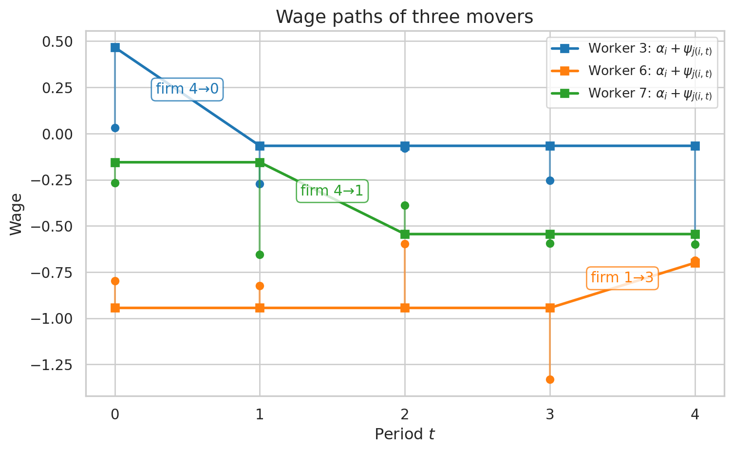
A small example

To make this concrete, we simulate a small dataset with \(n_j = 5\) firms, \(n_i = 10\) workers, and \(T = 5\) periods. We select three workers who change employer at least once and plot their wage paths. The lines show the systematic component \(\alpha_i + \psi_{j(i,t)}\), which shifts when a worker moves to a firm with a different \(\psi_j\). The vertical segments show the residual \(\epsilon_{it}\) added on top.

np.random.seed(7236)
p2 = Param(lambda1=0.559, rho=0.351, sigma=0.369, ng=10, nj=5, scale_alpha=0.550, scale_psi=0.317)
model = Model(p2)
dataset = model.simulate(10, 5)

# identify workers who move (work in at least 2 distinct firms)
movers = dataset.groupby('i')['j'].nunique()
mover_ids = movers[movers >= 2].index.tolist()[:3]

sns.set_theme(style="whitegrid")
palette = sns.color_palette("tab10", len(mover_ids))
fig, ax = plt.subplots(figsize=(8, 5))

for idx, worker_id in enumerate(mover_ids):
    wd = dataset[dataset['i'] == worker_id].sort_values('t')
    t = wd['t'].values
    j = wd['j'].values
    signal = wd['alpha'].values + wd['psi'].values
    y = wd['y'].values
    color = palette[idx]

    # line for alpha + psi
    ax.plot(t, signal, '-s', color=color, linewidth=2, markersize=6,
            label=f'Worker {worker_id}' + r': $\alpha_i + \psi_{{j(i,t)}}$')

    # vertical segments for the residual
    for tt, s, yy in zip(t, signal, y):
        ax.plot([tt, tt], [s, yy], color=color, linewidth=1.5, alpha=0.6)
        ax.plot(tt, yy, 'o', color=color, markersize=5, markeredgewidth=1.5)

    # annotate firm changes
    for k in range(1, len(t)):
        if j[k] != j[k-1]:
            mid_t = (t[k-1] + t[k]) / 2
            mid_y = (signal[k-1] + signal[k]) / 2
            ax.annotate(f'firm {j[k-1]}→{j[k]}',
                        xy=(mid_t, mid_y), fontsize=11, color=color,
                        ha='center', va='bottom',
                        bbox=dict(boxstyle='round,pad=0.3', fc='white', ec=color, alpha=0.8))

ax.set_xlabel('Period $t$', fontsize=12)
ax.set_ylabel('Wage', fontsize=12)
ax.set_xticks(range(5))
ax.set_title('Wage paths of three movers', fontsize=14)
ax.legend(fontsize=10)
plt.tight_layout()
plt.show()

Each line traces the systematic component \(\alpha_i + \psi_{j(i,t)}\) for one worker. When a worker changes firm, \(\psi_j\) changes and the line jumps — these discrete shifts are exactly what AKM exploits for identification. The small vertical segments (ending with an “x”) show the residual \(\epsilon_{it}\): the gap between the systematic part and the realized wage \(y_{it}\).

The raw data (below) shows the same information in tabular form.

Below is the raw data for the three movers shown in the plot. You can verify the firm changes and see how \(\psi\) shifts accordingly while \(\alpha\) stays constant within each worker.

dataset[dataset['i'].isin(mover_ids)].sort_values(by=['i', 't'])

	i	j	t	alpha	psi	epsilon	y
15	3	4	0	0.200241	0.266794	-0.435336	0.031699
16	3	0	1	0.200241	-0.266794	-0.206042	-0.272595
17	3	0	2	0.200241	-0.266794	-0.013334	-0.079887
18	3	0	3	0.200241	-0.266794	-0.187392	-0.253945
19	3	0	4	0.200241	-0.266794	-0.479064	-0.545617
30	6	1	0	-0.822050	-0.122147	0.147627	-0.796570
31	6	1	1	-0.822050	-0.122147	0.118952	-0.825244
32	6	1	2	-0.822050	-0.122147	0.346540	-0.597656
33	6	1	3	-0.822050	-0.122147	-0.386212	-1.330408
34	6	3	4	-0.822050	0.122147	0.011931	-0.687972
35	7	4	0	-0.422287	0.266794	-0.112416	-0.267909
36	7	4	1	-0.422287	0.266794	-0.499931	-0.655424
37	7	1	2	-0.422287	-0.122147	0.156630	-0.387803
38	7	1	3	-0.422287	-0.122147	-0.051122	-0.595555
39	7	1	4	-0.422287	-0.122147	-0.054636	-0.599069

How did we estimate AKM?

The AKM estimator recovers the worker and firm fixed effects from the wage equation \(y_{it} = \alpha_i + \psi_{j(i,t)} + \epsilon_{it}\) by ordinary least squares. We walk through the steps using a fresh simulated dataset with 1,000 workers, 100 firms, and 5 periods.

Step 1: Simulate and build the design matrix

We simulate a new dataset and restrict it to the largest connected set of firms (connected through worker mobility). We then construct the design matrix \(X = [A_f \; A_w]\), where \(A_f\) is an \(N \times (n_j - 1)\) matrix of firm indicators (one firm is normalized to zero) and \(A_w\) is an \(N \times n_i\) matrix of worker indicators.

Step 2: Solve by OLS

The OLS estimator solves the normal equations \(X'X \hat{\beta} = X'y\). The solution vector \(\hat{\beta}\) contains the estimated firm effects \(\hat{\psi}_j\) (first \(n_j - 1\) entries) and the estimated worker effects \(\hat{\alpha}_i\) (remaining entries). We then recover the fitted values by multiplying back through the indicator matrices.

np.random.seed(6344)
model = Model(lambda1=0.559, rho=0.351, sigma=0.369, ng=10, nj=100, scale_alpha=0.550, scale_psi=0.317)
dataset = model.simulate(1_000, 5, connected=True)

# build the design matrix X = [Af, Aw]
M, Af, Aw = data_to_matrix(dataset)

# solve the normal equations: (X'X) beta = X'y
MM = M.T @ M
x = np.linalg.solve(MM, M.T @ dataset['y'].to_numpy())

# recover fitted effects for each observation
psi_hat = Af @ x[:Af.shape[1]]
alpha_hat = Aw @ x[Af.shape[1]:]

Largest connected component: 100

Step 3: Compare estimates to truth

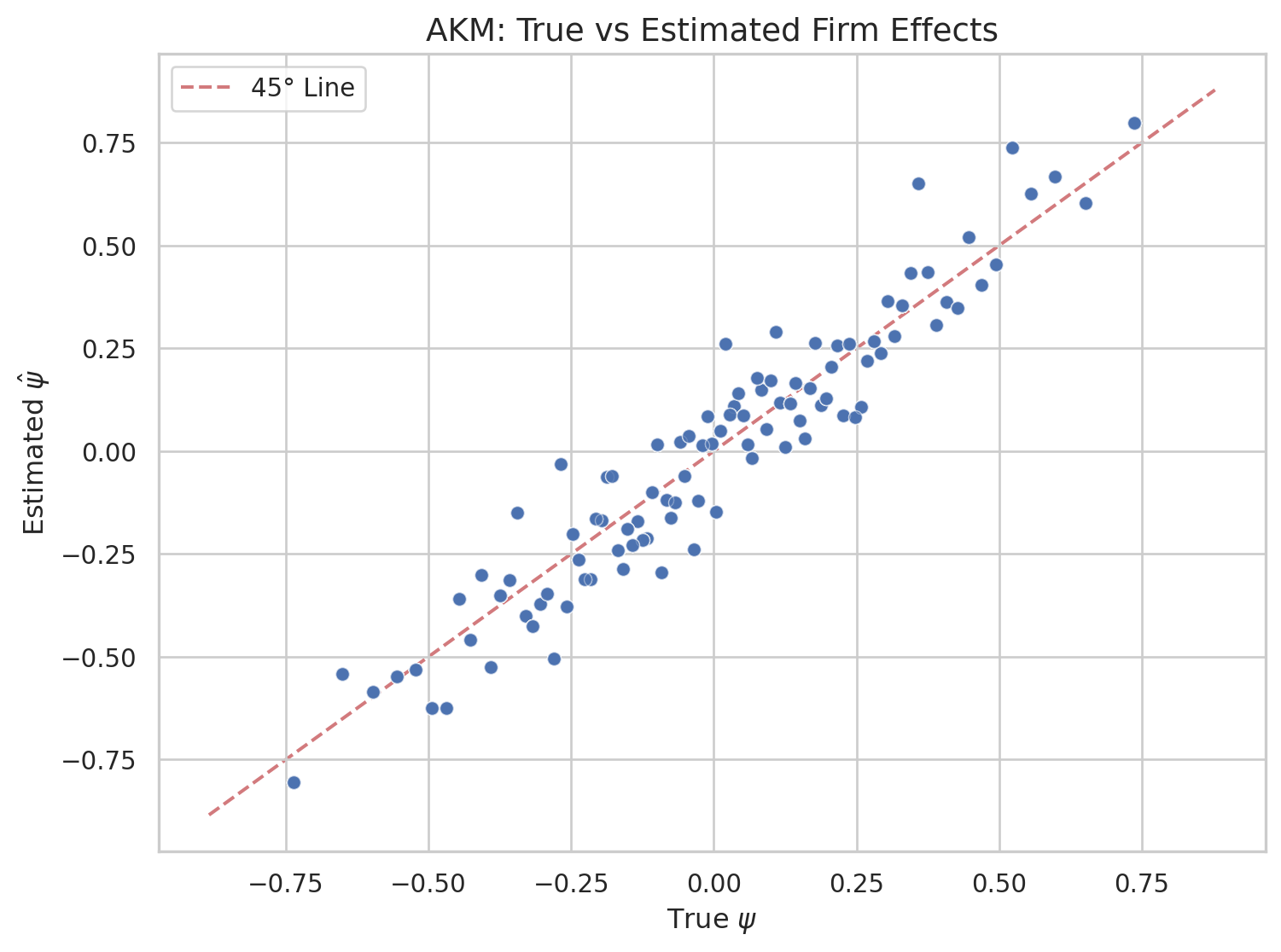
Since we simulated the data, we can compare the estimated \(\hat{\psi}_j\) to the true \(\psi_j\). The scatter plot below shows each observation’s true firm effect on the horizontal axis and the estimated value on the vertical axis. Points close to the 45-degree line indicate accurate recovery; dispersion around it reflects estimation noise — particularly for firms with few worker-period observations.

sns.set_theme(style="whitegrid")
plt.figure(figsize=(8, 6))

# demean estimated firm effects (mean level is not identified)
psi_hat_dm = psi_hat - psi_hat.mean()

plt.scatter(dataset['psi'].to_numpy(), psi_hat_dm, alpha=0.4, edgecolors='w', linewidth=0.5)

lims = [np.min([plt.xlim(), plt.ylim()]), np.max([plt.xlim(), plt.ylim()])]
plt.plot(lims, lims, 'r--', alpha=0.75, zorder=0, label='45° Line')

plt.xlabel(r'True $\psi$', fontsize=12)
plt.ylabel(r'Estimated $\hat{\psi}$', fontsize=12)
plt.title('AKM: True vs Estimated Firm Effects', fontsize=14)
plt.legend()
plt.tight_layout()
plt.show()

Estimating AKM with the zig-zag algorithm

The direct OLS approach above solves the full normal equations in one shot. This requires inverting a very large matrix (of dimension \(n_i + n_j\)), which can be prohibitive with millions of workers and firms. An alternative is the zig-zag (or alternating projections) algorithm, which iterates between two simple steps:

Update worker effects: holding \(\hat\psi_j\) fixed, compute each \(\hat\alpha_i\) as the mean residual across that worker’s observations: \[\hat{\alpha}_i \leftarrow \frac{1}{T_i} \sum_{t} \big(y_{it} - \hat{\psi}_{j(i,t)}\big)\]
Update firm effects: holding \(\hat\alpha_i\) fixed, compute each \(\hat\psi_j\) as the mean residual across that firm’s observations: \[\hat{\psi}_j \leftarrow \frac{1}{N_j} \sum_{(i,t):\, j(i,t)=j} \big(y_{it} - \hat{\alpha}_i\big)\]

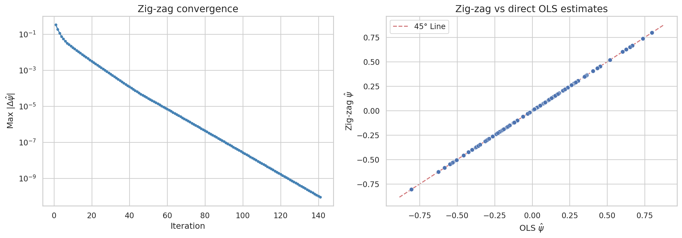
These two steps are repeated until convergence. Each step is a simple group-mean computation, making this approach very scalable. We demonstrate it on the same simulated dataset used above.

def compute_akm_zigzag(dataset, max_iter=200, tol=1e-10):
    """Estimate AKM via alternating projections (zig-zag)."""
    y = dataset['y'].to_numpy()
    worker = dataset['i'].to_numpy()
    firm = dataset['j'].to_numpy()

    # initialize firm effects to zero
    nj = len(np.unique(firm))
    psi_hat = np.zeros(nj)
    history = []

    for iteration in range(max_iter):
        # Step 1: update worker effects holding firm effects fixed
        residual_w = y - psi_hat[firm]
        alpha_hat_vals = pd.Series(residual_w).groupby(worker).transform('mean').to_numpy()

        # Step 2: update firm effects holding worker effects fixed
        residual_f = y - alpha_hat_vals
        psi_new = pd.Series(residual_f).groupby(firm).mean().to_numpy()

        # check convergence
        change = np.max(np.abs(psi_new - psi_hat))
        history.append(change)
        psi_hat = psi_new

        if change < tol:
            print(f"Converged after {iteration + 1} iterations (max change = {change:.2e})")
            break
    else:
        print(f"Stopped after {max_iter} iterations (max change = {change:.2e})")

    # recover per-observation fitted values
    psi_hat_obs = psi_hat[firm]
    alpha_hat_obs = y - psi_hat_obs
    alpha_hat_obs = pd.Series(alpha_hat_obs).groupby(worker).transform('mean').to_numpy()

    return alpha_hat_obs, psi_hat_obs, history

alpha_hat_zz, psi_hat_zz, convergence_history = compute_akm_zigzag(dataset)

Converged after 141 iterations (max change = 9.04e-11)

We can plot the convergence of the algorithm (the maximum change in \(\hat\psi\) across iterations) and compare the zig-zag estimates to the direct OLS estimates from earlier.

sns.set_theme(style="whitegrid")
fig, axes = plt.subplots(1, 2, figsize=(14, 5))

# Left panel: convergence
axes[0].semilogy(range(1, len(convergence_history) + 1), convergence_history, '-o', markersize=3, color='steelblue')
axes[0].set_xlabel('Iteration', fontsize=12)
axes[0].set_ylabel(r'Max $|\Delta \hat{\psi}|$', fontsize=12)
axes[0].set_title('Zig-zag convergence', fontsize=14)

# Right panel: zig-zag vs OLS estimates
psi_hat_zz_dm = psi_hat_zz - psi_hat_zz.mean()
axes[1].scatter(psi_hat_dm, psi_hat_zz_dm, alpha=0.4, edgecolors='w', linewidth=0.5)
lims = [np.min([axes[1].get_xlim(), axes[1].get_ylim()]),
        np.max([axes[1].get_xlim(), axes[1].get_ylim()])]
axes[1].plot(lims, lims, 'r--', alpha=0.75, zorder=0, label='45° Line')
axes[1].set_xlabel(r'OLS $\hat{\psi}$', fontsize=12)
axes[1].set_ylabel(r'Zig-zag $\hat{\psi}$', fontsize=12)
axes[1].set_title('Zig-zag vs direct OLS estimates', fontsize=14)
axes[1].legend()

plt.tight_layout()
plt.show()

print(f"Max absolute difference between OLS and zig-zag: {np.max(np.abs(psi_hat_dm - psi_hat_zz_dm)):.2e}")

Max absolute difference between OLS and zig-zag: 6.05e-10

The left panel shows that the maximum update to any firm effect shrinks geometrically, reaching machine precision in relatively few iterations. The right panel confirms that the zig-zag and direct OLS estimates are numerically identical — both methods solve the same least-squares problem, just via different algorithms. The zig-zag approach scales much better to large datasets because each iteration only requires computing group means, avoiding the construction and inversion of the full \(X'X\) matrix.